March 24th, 2025

Postulate IV: Probability for a measurement

Author: Quentin Stern
Editor: Joshua Straub

The full scripts presented in this post are available at these links: MATLAB, Python

In the previous post, we saw that for any state $\ket{\psi}$ , measuring the observable $A$ can only result in one of the eigenvalues $a_n$ of the Hermitian operator $\hat{A}$ associated with $A$ . We concluded by asking what could be the probability of measuring one eigenvalue $a_n$ rather than another one $a_m$ .

An eigenvalue $a_n$ of $\hat{A}$ is associated with an eigenvector $\ket{n}$ . Now, remember that, by the first postulate, if the system is initially prepared in an arbitrary state $\ket{\psi}$ , the probability of finding it in state $\ket{n}$ is given by $p_{\psi\rightarrow n}=\vert\braket{n\vert\psi}\vert^2$ . Postulates 1 to 3 taken together point towards the idea that the probability $p(a_{n})$ of measuring the eigenvalue $a_n$ for the system prepared in state $\ket{\psi}$ is equal to the probability $p_{\psi\rightarrow n}$ of finding the system in the eigenstate $\ket{n}$ associated with $a_n$ . In other words, the more likely we are to find the system in a state $\ket{n}$ , the more likely we are to measure the eigenvalue $a_n$ associated with $\ket{n}$ . That’s precisely what the fourth postulate states.

Formulation of the postulate

Postulate IV: For a system in state $\ket{\psi}$ , the probability of measuring the eigenvalue $a_n$ of operator $\hat{A}$ is given by

(1) $\begin{equation*}p(a_{n})=\sum_{k=1}^{g_n}\vert\braket{k\vert\psi}\vert^2,\end{equation*}$

where $g_n$ is the degeneracy of $a_n$ and the states $\ket{k}$ are the $g_n$ eigenstates associated with $a_n$ . If $a_n$ is non-degenerate, that is, if $g_n=1$ , we have

(2) $\begin{equation*}p_{a_n }=\vert\braket{n\vert\psi}\vert^2,\end{equation*}$

where $\ket{n}$ is the single eigenstate associated with $a_n$ .

Note that we restrict the formulation of the postulates to quantum systems with a discrete spectrum and so we use a discrete summation in the formulation of the fourth postulate. This is always appropriate for describing spin states. On the contrary, it is not appropriate to describe harmonic oscillators, where the potential is a function of the special coordinates, like the orbitals of an electron in an atom. Still, even in this case, we can often treat the spin states of the electron independently of its spatial properties, and the above formulation remains appropriate.

If a single spin is in state $\ket{\psi}=\ket{\alpha}$ , then Eq. 2 predicts that we have probabilities $p_{\alpha}=1$ and $p_{\beta}=0$ to measure angular momenta $+1/2$ and $-1/2$ , respectively (expressed setting $\hbar = 1$ ). Conversely, if a single spin is in state $\ket{\psi}=\ket{\beta}$ , then Eq. 2 predicts that we have probabilities $p_{\alpha}=0$ and $p_{\beta}=1$ to measure angular momenta $+1/2$ and $-1/2$ , respectively. If the system is in a superposition of states, for example

(3) $\begin{equation*}\ket{\pm x}=\frac{1}{\sqrt{2}}\left(\ket{\alpha}\pm\ket{\beta}\right),\end{equation*}$

or

(4) $\begin{equation*}\ket{\pm y}=\frac{1}{\sqrt{2}}\left(\ket{\alpha}+\pm i\ket{\beta}\right),\end{equation*}$

then Eq. 2 predicts that there is an equal probability to measure both eigenvalues

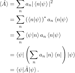
(5) $\begin{equation*}p_{\alpha}=p_{\beta}=\left(\frac{1}{\sqrt{2}}\right)^2=\frac{1}{2}.\end{equation*}$

Expectation value

An important consequence of the fourth postulate is that, if we repeat the same measurement of the observable $A$ on many identical quantum systems (or many times on a system prepared in the same state), then the expectation value of the measurement is

(6) $\begin{align*}\braket{\hat{A}}=\braket{\psi\vert\hat{A}\vert\psi}.\end{align*}$

Details on the calculations

From the first to the second line, we the fact this identity of complex numbers: $\vert z\vert^2 =z^*z$ . From the second to the third line, we apply the complex transpose. From the third to the fourth line, we take out of the sum the element that do not depend on $n$ . Finally, we recognize that the sum in the fourth line is the expression for the operator $\hat{A}$ that we gave in the previous post.

$\begin{align*}\braket{\hat{A}} &= \sum_n a_n \vert\braket{n\vert\psi}\vert^2 \\&= \sum_n\left(\braket{n\vert\psi}\right)^* a_n \braket{n\vert\psi} \\&= \sum_n \braket{\psi\vert n} a_n\braket{n\vert\psi}\\&= \bra{\psi}\left( \sum_n a_n \ket{n}\bra{n} \right) \ket{\psi}\\&=\braket{\psi\vert\hat{A}\vert\psi}.\label{Eq_ExpectationValue}\end{align*}$

Note that the development we show here is only valid for non-degenerate operators. However, it can be shown that the relation of Eq. 6 holds for any Hermitian operator $\hat{A}$ .

In NMR experiments, the recorded signal is the collective effect of many identical spin systems. Therefore, the measurement always results in an expectation value and does not give access to the state of an individual spin system. This is a key aspects of NMR experiments and we will come back to that in future posts.

Single spin in a magnetic field

For a spin in state $\ket{\alpha}$ , the expectation value of the quantity $I_z$ is $\braket{\hat{I}_z} = p_{\alpha}(+1/2)+p_{\beta}(-1/2)=+1/2$ , or using the notation of Eq. 6,

(7) $\begin{align*}\braket{\hat{I}_z}&=\braket{\alpha\vert\hat{I}_z\vert\alpha}\\&=\begin{pmatrix}1 &&0\end{pmatrix}\begin{pmatrix}+1/2 && 0\\0 && -1/2\end{pmatrix}\begin{pmatrix}1 \\0\end{pmatrix}\\&=+1/2\end{align*}$

Similarly, the angular momentum along the $z$ -axis of the spin in the superposition state of Eq. 3 has an expectation value $\braket{\hat{I}_z}=p_{\alpha}(+1/2)+p_{\beta}(-1/2)=0$ because both states are equally probable. Using the notation of Eq. 6

(8) $\begin{align*}\braket{\hat{I}_z}&=\braket{x\vert\hat{I}_z\vert x}\\&=\frac{1}{\sqrt{2}}\begin{pmatrix}1 && 1 \end{pmatrix}\begin{pmatrix}+1/2 && 0\\0 && -1/2\end{pmatrix}\frac{1}{\sqrt{2}}\begin{pmatrix}1 \\1\end{pmatrix}\\&=0.\end{align*}$

As mentioned in the previous post, the states $\ket{x}$ and $\ket{y}$ that we defined correspond to the state having its angular momentum oriented along the $x$ and $y$ axes, respectively. This can be verified by computing the expectation value of $\ket{x}$ for operator $\hat{I}_x$ and $\ket{y}$ for operator $\hat{I}_y$

(9) $\begin{align*}\braket{\hat{I}_x}&=\braket{x\vert\hat{I}_x\vert x}\\&=\frac{1}{\sqrt{2}}\begin{pmatrix}1 && 1 \end{pmatrix}\begin{pmatrix}0 &&+1/2\\+1/2 && 0\end{pmatrix}\frac{1}{\sqrt{2}}\begin{pmatrix}1 \\1\end{pmatrix}\\&=+\frac{1}{2}.\end{align*}$

(10) $\begin{align*}\braket{\hat{I}_y}&=\braket{y\vert\hat{I}_y\vert y}\\&=\frac{1}{\sqrt{2}}\begin{pmatrix}1 && -i \end{pmatrix}\begin{pmatrix}0 &&-i/2\\+i/2 && 0\end{pmatrix}\frac{1}{\sqrt{2}}\begin{pmatrix}1 \\-i\end{pmatrix}\\&=+\frac{1}{2}.\end{align*}$

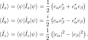
For a single spin in an arbitrary state $\ket{\psi} = c_\alpha\ket{\alpha}+c_\beta\ket{\beta}$ , with $\vert c_\alpha\vert^2+\vert c_\beta\vert^2=1$ , the expectation value in the three directions are

(11) $\begin{equation*}\begin{split} \braket{\hat{I}_x}&=\braket{\psi\vert\hat{I}_x\vert \psi} =\frac{1}{2}\left(c_\alpha c_\beta^*+c_\alpha^* c_\beta\right) \\ \braket{\hat{I}_y}&=\braket{\psi\vert\hat{I}_y\vert \psi} =\frac{i}{2}\left(c_\alpha c_\beta^*-c_\alpha^* c_\beta\right) \\ \braket{\hat{I}_z}&=\braket{\psi\vert\hat{I}_z\vert \psi} =\frac{1}{2}\left(\vert c_\alpha\vert^2 -\vert c_\beta\vert^2\right). \end{split}\end{equation*}$

The expectations values of angular momentum operators can be computed in a computer program in the following way.

MATLAB
Python
Mathematica

% Definition of the angular momentum operators
Ix = [0  +1;+1  0]/2;
Iy = [0  -1;+1  0]*1i/2;
Iz = [+1  0; 0 -1]/2;

% Definition of states
alpha = [1; 0];          % Pure state
x     = [1; 1]/sqrt(2);  % Superposition
y     = [1; 1]/sqrt(2);  % Superposition
psi   = rand(2,1)+1i*rand(2,1);  % Arbitrary
psi   = psi/norm(psi);

% Expectations values of the alpha state all Cartesian coordinates
Ix_alpha = alpha'*Ix*alpha;
Iy_alpha = alpha'*Iy*alpha;
Iz_alpha = alpha'*Iz*alpha;

% Expectations values of the x state all Cartesian coordinates
Ix_x = x'*Ix*x;
Iy_x = x'*Iy*x;
Iz_x = x'*Iz*x;

% Expectations values of the y state all Cartesian coordinates
Ix_y = y'*Ix*y;
Iy_y = y'*Iy*y;
Iz_y = y'*Iz*y;

% Expectations values of the psi state all Cartesian coordinates
Ix_psi = psi'*Ix*psi;
Iy_psi = psi'*Iy*psi;
Iz_psi = psi'*Iz*psi;

# Definition of kets
alpha = np.array([1, 0])
x     = np.array([1, 1])/np.sqrt(2)
y     = np.array([1, 1j])/np.sqrt(2)
psi   = np.random.rand(2)+1j*np.random.rand(2)
psi   = psi/np.linalg.norm(psi)

# Definition of the angular momentum operators
Ix = np.array([[0,  +1/2],[ +1/2, 0]])
Iy = np.array([[0, -1j/2],[+1j/2, 0]])
Iz = np.array([[+1/2,  0],[0,  -1/2]])

# Function for computing expectation of an operator op and and a ket
def ExpVal(op,ket):
    return np.dot(np.conjugate(ket),np.dot(op,ket));

# Expectations values of the alpha state all Cartesian coordinates
Ix_alpha = ExpVal(Ix, alpha)
Iy_alpha = ExpVal(Iy, alpha)
Iz_alpha = ExpVal(Iz, alpha)

# Expectations values of the x state all Cartesian coordinates
Ix_x     = ExpVal(Ix, x)
Iy_x     = ExpVal(Iy, x)
Iz_x     = ExpVal(Iz, x)

# Expectations values of the y state all Cartesian coordinates
Ix_y     = ExpVal(Ix, y)
Iz_y     = ExpVal(Iy, y)
Iy_y     = ExpVal(Iz, y)

# Expectations values of the psi state all Cartesian coordinates
Ix_psi   = ExpVal(Ix, psi)
Iy_psi   = ExpVal(Iy, psi)
Iz_psi   = ExpVal(Iz, psi)

none

Bloch sphere

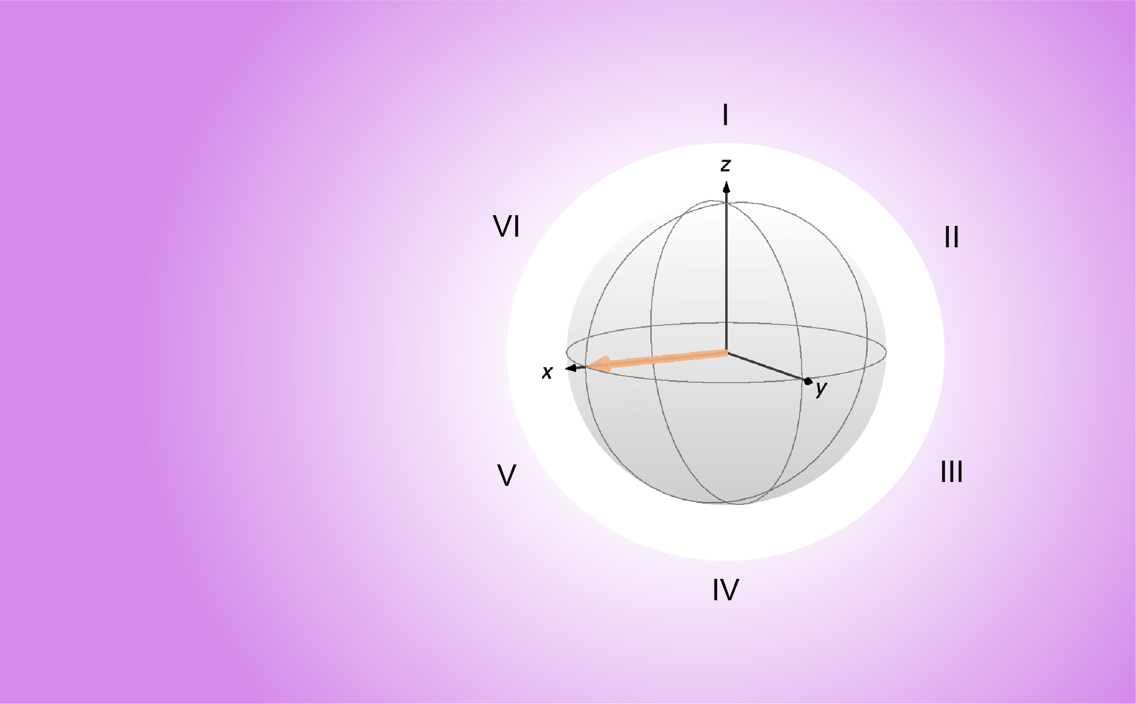
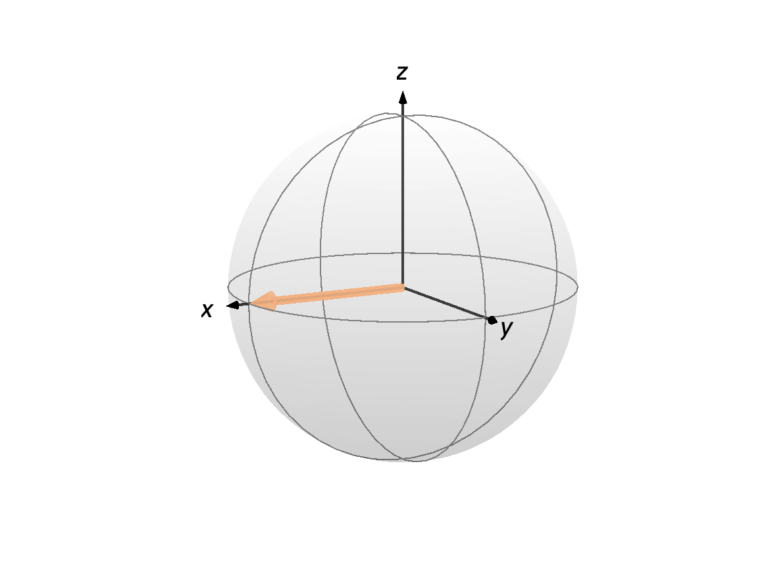
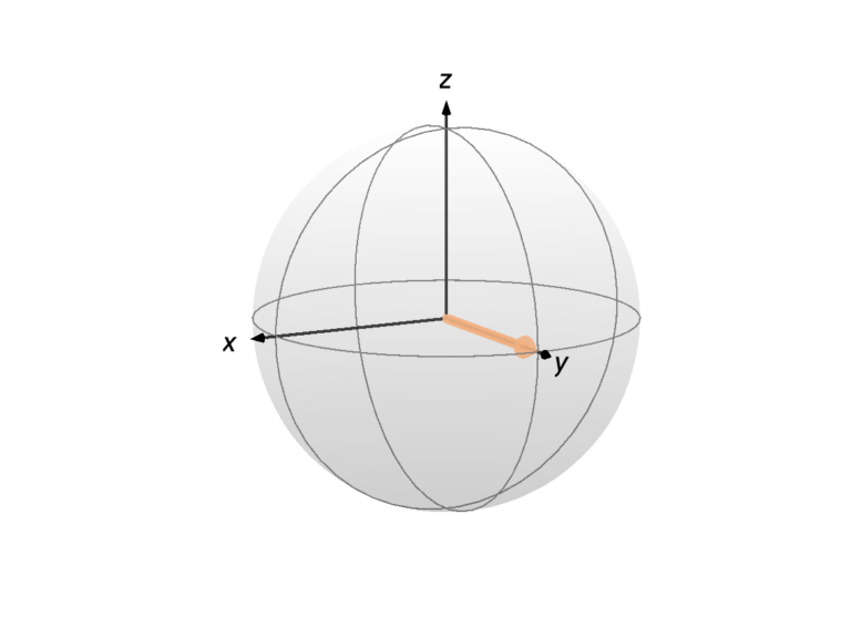
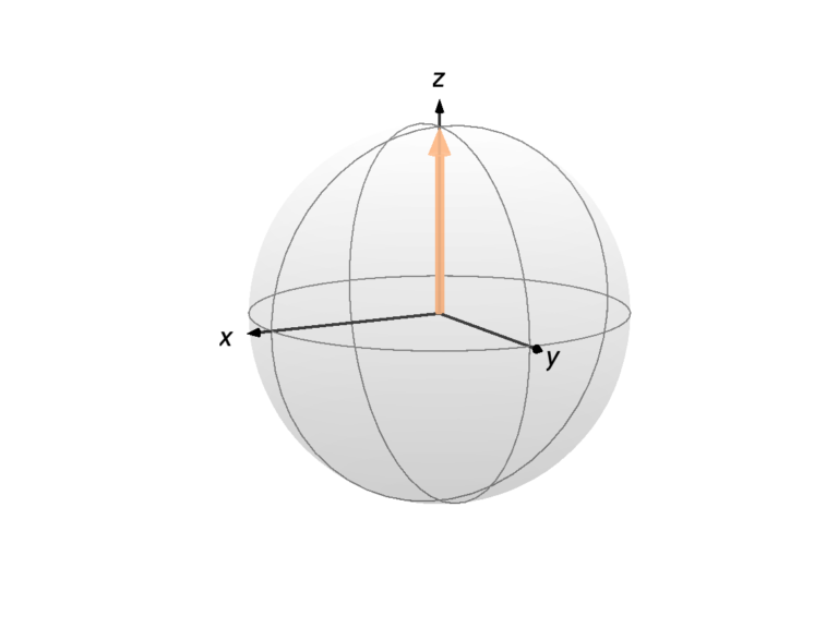
The states $\ket{x}$ and $\ket{y}$ defined above and the state $\ket{z}=\ket{\alpha}$ correspond to the spin having its angular momentum along all three Cartesian coordinates. That’s the basis of the so-called Bloch sphere, a visual representation of the spin state as a point on a sphere, as shown in the images below, where the spin is represented by a colored arrow. Any state of a single spin 1/2 can be represented as a point on the Bloch sphere (up to the global phase, but we’ll come back to that in the post on the sixth postulate).

Conclusion

It is post, we talked about the probability of obtaining a certain eigenvalue $a_n$ of n operator $\hat{A}_n$ when measuring $\hat{A}_n$ on a quantum mechanical system $\ket{\psi}$ . In the next post, we will talk about the consequences of measuring this eigenvalue, the so-called collapse of the wave function.

To previous post:
Postulates II & III

To next post:
Postulate V

Postulate IV: Probability for a measurement

Formulation of the postulate

Expectation value

Details on the calculations

Single spin in a magnetic field

Bloch sphere

Conclusion

Leave a Reply Cancel reply

Artist Credit:

Contact:

Website designed and developed by:

Postulate IV: Probability for a measurement

Formulation of the postulate

Expectation value

Details on the calculations

Single spin in a magnetic field

Bloch sphere

Conclusion

Leave a Reply Cancel reply

Artist Credit:

Contact:

Website designed and developed by:

Quantum Insights