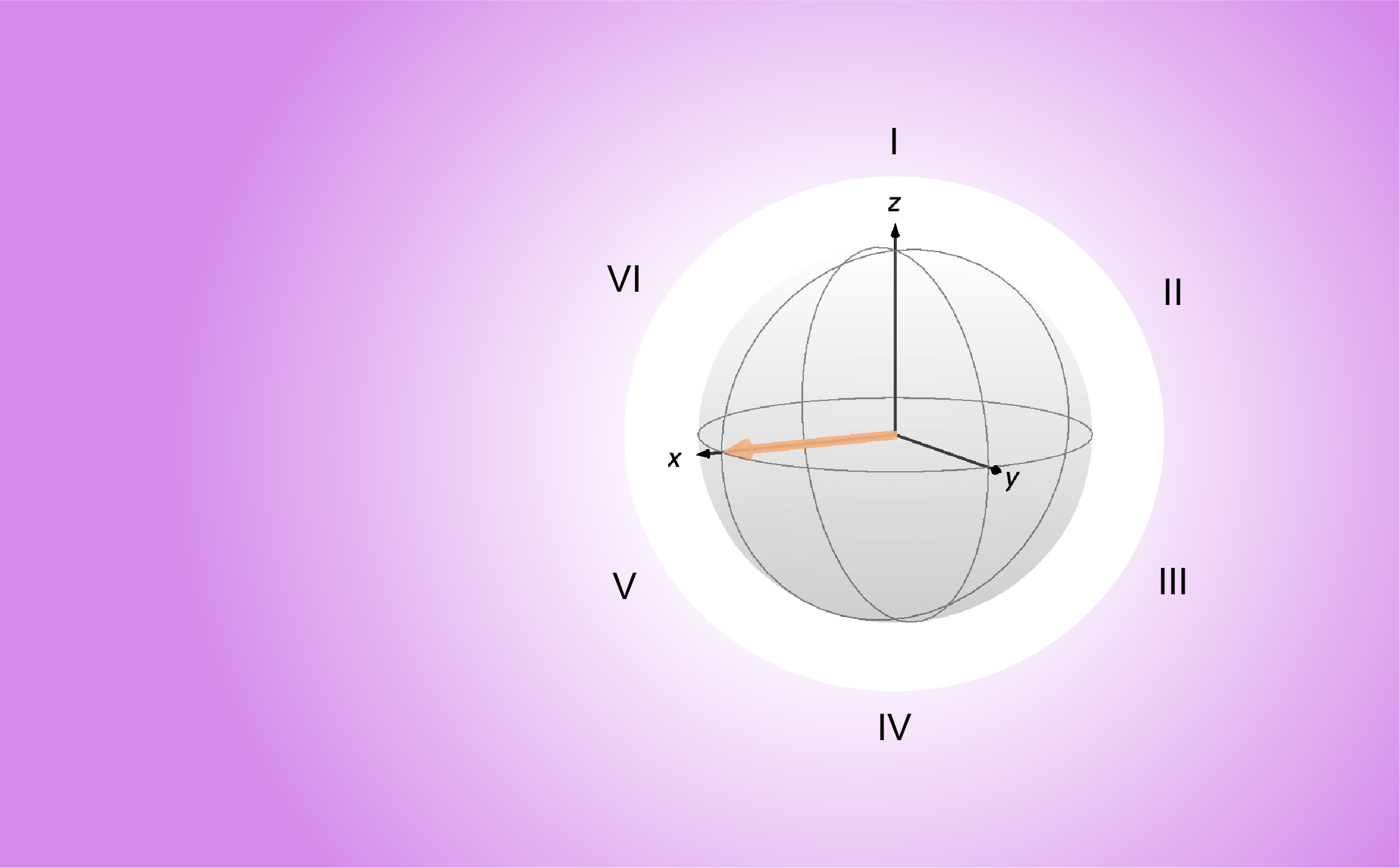
The full scripts presented in this post are available at these links: MATLAB, Python
To develop the framework of quantum mechanics in the early 20th century, pioneer scientists had to question our knowledge about the world. They had to ask themselves what a measurement and an observer are, and how they interact. When Newton introduced his famous laws of motion, he didn’t have to ask such questions: if an apple falls from a tree, the observer can look at the apple’s trajectory and the very fact of looking at it does not modify the course of its fall. In quantum mechanics, things are more complicated. The system and its observer can’t be so trivially separated. This is why the postulates of quantum mechanics were introduced: they define mathematically some key concepts like what a “system” is, what a “measurement” is, how does the system evolve in time, and, more surprisingly, the consequences of performing a measurement on the system.
Now let’s start with the first postulate, which defines what a quantum mechanical system is. It can be formulated as follows:
Postulate I: A quantum mechanical system is fully described by a wave function
. The space of all possible states
of the system is a complex Hilbert space denoted
. If the system is in state
, the probability to find it in state
is given by
(1)
where
denotes the scalar product on
.
A Hilbert space is a vector space with an inner product or scalar product. ![]() is an element of this space, also called a vector.
is an element of this space, also called a vector.
Although Hilbert spaces are a more general mathematical concept, for the purpose of describing spin dynamics, we’ll only need to deal with an ![]() -dimensional vector space
-dimensional vector space ![]() (where
(where ![]() is finite) with the usual scalar product (or dot product or inner product) defined by
is finite) with the usual scalar product (or dot product or inner product) defined by

which corresponds to the element-by-element multiplication of the elements of ![]() and the complex conjugate elements of
and the complex conjugate elements of ![]() . In a space where an scalar product is defined, the notion of length or norm of a vector
. In a space where an scalar product is defined, the notion of length or norm of a vector ![]() naturally follows
naturally follows

which is a positive number, linear with ![]() , as a length should be.
, as a length should be.
The object ![]() is called a “bra” while
is called a “bra” while ![]() is called a “ket”; together they form a “bra-ket”, which corresponds to the scalar product on
is called a “ket”; together they form a “bra-ket”, which corresponds to the scalar product on ![]() . While the ket represents the state of the system, the bra is the Hermitian conjugate of the ket
. While the ket represents the state of the system, the bra is the Hermitian conjugate of the ket
(2) ![]()
a complementary mathematical object which allows us to compute information on the system. Note that, to write Eq. 1, we have implicitly assumed that the states were normalized, i.e.,
(3) ![]()
which will be the case throughout this post series.
In general, the wave function is the product of several properties
(4) ![]()
where ![]() denotes the Kronecker product of the states. If
denotes the Kronecker product of the states. If ![]() lives in the space
lives in the space ![]() ,
, ![]() and
and ![]() live in subspaces of
live in subspaces of ![]() As stated in the first post of this series, we only need to take into account the spin part of the wavefunction to describe NMR experiments. We will therefore describe all states assuming
As stated in the first post of this series, we only need to take into account the spin part of the wavefunction to describe NMR experiments. We will therefore describe all states assuming ![]() .
.
Now let us assume that we are Walther Gerlach and we have just performed the first Stern-Gerlach experiment. We know that a silver atom subject to a magnetic field can take two values of the spin angular momentum, which arises due to the unpaired electron of the silver atom: ![]() and
and ![]() , when parallel or antiparallel with the magnetic field
, when parallel or antiparallel with the magnetic field ![]() aligned along
aligned along ![]() , respectively. These two values are associated with the magnetic moments
, respectively. These two values are associated with the magnetic moments
(5) ![]()
where ![]() is the gyromagnetic ratio of the spin (which is negative in the case of the electron). These magnetic moments are associate with the energies
is the gyromagnetic ratio of the spin (which is negative in the case of the electron). These magnetic moments are associate with the energies
(6) ![]()
The states where the spin is parallel or antiparallel with the magnetic field are often called ![]() and
and ![]() , respectively, and are referred to as the Zeeman states. As we will see in more detail in the next posts, the states
, respectively, and are referred to as the Zeeman states. As we will see in more detail in the next posts, the states ![]() and
and ![]() are sufficient to fully describe an isolated spin 1/2, i.e., they form a basis of
are sufficient to fully describe an isolated spin 1/2, i.e., they form a basis of ![]() , referred to as the Zeeman basis
, referred to as the Zeeman basis ![]() . Going back to the first postulate, this implies that all possible states of an isolated spin 1/2 are spanned by
. Going back to the first postulate, this implies that all possible states of an isolated spin 1/2 are spanned by ![]() and can be written as linear combinations of the basis states
and can be written as linear combinations of the basis states
(7) ![]()
where ![]() and
and ![]() are complex coefficients satisfying the normalization condition
are complex coefficients satisfying the normalization condition
(8) ![]()
To compute the norm of the ![]() (first equality in Eq. 8), we made use of an important property of basis states, the orthonormality, i.e. orthogonal and normalized. Basis states are always orthogonal, that is, the scalar product between two different basis states is 0. It is often convenient to define them so that they are normalized, that is, they have a norm of 1. For any two basis states
(first equality in Eq. 8), we made use of an important property of basis states, the orthonormality, i.e. orthogonal and normalized. Basis states are always orthogonal, that is, the scalar product between two different basis states is 0. It is often convenient to define them so that they are normalized, that is, they have a norm of 1. For any two basis states ![]() and
and ![]() , the condition of orthonormality can be expressed as
, the condition of orthonormality can be expressed as
(9) ![]()
where ![]() is the Kronecker delta. Look at the details below to understand how we used the orthonormality of the basis states to calculate the norm of
is the Kronecker delta. Look at the details below to understand how we used the orthonormality of the basis states to calculate the norm of ![]() . It’s a common and important type of calculation.
. It’s a common and important type of calculation.
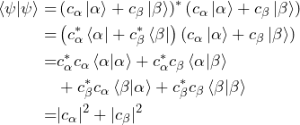
In the first line, we insert the expression for the ket (Eq. 7) and apply the definition of the bra (Eq. 2). In the first to the second line, we apply the Hermitian conjugate in the parentheses. In the second to the third line, we distribute the product. From the third to the forth, we make use of the fact that the states are orthonormal and use the property of complex numbers ![]() .
.

More generally, any state of a quantum mechanical system can be written as a linear combination of the basis states
(10) ![]()
The matrix representation of quantum mechanics consists of associating the basis states with vectors. In this representation, a state ![]() is identified with a column vector
is identified with a column vector
(11) ![]()
In programming terms, one can use standard linear algebra notation to represent these states (in the case of Python, you need the library Numpy).
% Definition of kets for alpha and beta states
ket_alpha = [1; 0];
ket_beta  = [0; 1];
# Required package for numerical calculations
import numpy as np
# Definition of kets for alpha and beta states
ket_alpha = np.array([1, 0])
ket_beta = np.array([0, 1])noneAn arbitrary state following the definition in Eq. 7 can be generated as follows.
% Definition of an arbitrary linear combination
% of alpha and beta
ket_psi = rand(2,1)+1i*rand(2,1);

% Normalization
ket_psi = ket_psi/norm(ket_psi);
# Definition of an arbitrary linear combination
# of alpha and beta
ket_psi = np.random.rand(2)+1j*np.random.rand(2)
# Normalization
ket_psi = ket_psi/np.linalg.norm(ket_psi)
display(np.linalg.norm(ket_psi))
display(ket_psi)noneIn the matrix representation, the Hermitian conjugate of the state is the conjugate transpose of the vector representing the state (as expressed in Eq. 2).
bra_alpha = ket_alpha';
bra_beta  = ket_beta';
bra_psi   = ket_psi';
bra_alpha = np.conjugate(ket_alpha)
bra_beta = np.conjugate(ket_beta)
bra_psi = np.conjugate(ket_psi)noneUsing the first postulate, we find that there is a null probability of finding the system in the ![]() state if it is known to be in the
state if it is known to be in the ![]() state and vice versa,
state and vice versa,
(12) ![]()
but a probability of 1 of finding the system in the ![]() state if it is initially in
state if it is initially in ![]() and the same for
and the same for ![]() ,
,
(13) ![]()
which should not be too surprising. This can be expressed programmatically as below.
paa = abs(bra_alpha*ket_alpha)^2;
pab = abs(bra_alpha*ket_beta)^2;
pba = abs(bra_beta*ket_alpha)^2;
pbb = abs(bra_beta*ket_beta)^2;
paa = np.square(np.absolute(np.dot(bra_alpha,ket_alpha)))
pab = np.square(np.absolute(np.dot(bra_alpha,ket_beta)))
pba = np.square(np.absolute(np.dot(bra_beta,ket_alpha)))
pbb = np.square(np.absolute(np.dot(bra_beta,ket_beta)))
# Convert singleton into scalar
paa = paa.item(0)
pab = pab.item(0)
pba = pba.item(0)
pbb = pbb.item(0)noneFor the general state of Eq. 7, we find the following probabilities to be in the ![]() or
or ![]() states
states
(14) 
and
(15) 
which shows that the probability to find ![]() in state
in state ![]() is given by the square of the amplitude of
is given by the square of the amplitude of ![]() in
in ![]() . The coefficients above can be computed in the following way.
. The coefficients above can be computed in the following way.
p_alpha = abs(bra_alpha* ket_psi)^2;
p_beta  = abs(bra_beta* ket_psi)^2;
palpha = np.square(np.absolute(np.dot(bra_alpha,ket_psi)))
pbeta = np.square(np.absolute(np.dot(bra_beta,ket_psi)))
# Convert singleton into scalar
palpha = palpha.item(0)
pbeta = pbeta.item(0)noneIn the lines above, we have stated one of these facts of Quantum Mechanics that are hard to swallow: a system can be in multiple states at the same time. What this means in practice will only become clearer once we introduce the next postulates regarding measurements on quantum mechanical systems. So, read on to the next posts to learn more!