Hello and welcome back! Today we are going to be introducing the basics of optically detected magnetic resonance (ODMR) with NV centers. In a previous post, we introduced the electronic energy structure of the NV (technically NV ) center. We saw that under optical excitation, there are multiple relaxation pathways, both radiative and non-radiative. The
  state was more likely to undergo the radiative relaxation pathway and emit a photon as compared to the
  state. This spin-dependent fluorescence of the NV center is what allows for ODMR, where the relative populations of spin states can be measured via the intensity of light emission from the center.
In this post, we will begin by explaining the state preparation and readout, and then move on to some simple (but still very useful) experiments. Hopefully, this introduction to ODMR provides the reader with the fundamentals of the technique, and the tools to be able to understand more complex experiments that may be encountered in the literature and in research environments.
As discussed in our post on the NV electronic energy structure, optically excited NV electronic states have both radiative and non-radiative relaxation pathways. The likelihood of relaxation occurring via each of these pathways from the excited triplet state depends on the  state of the triplet. This dependence on spin state has two significant consequences.
First, optical excitation causes the conversion of  states into at a greater rate than the opposite direction (
 ). This rate difference means that we can spin polarize the NV center into the state via optical excitation with a laser at the proper wavelength (commonly 532 nm lasers are used). In reality, one does not achieve
  spin polarization, but the achievable spin polarization far exceeds thermal polarization, and thus is significant hyperpolarization – values up to
  have been reported in crystal diamonds (Waldherr et al., PRL 2011).
Second, the state is more likely to relax via a radiative pathway than the states. For all of these spin states, the (spin-conserving) radiative decay from the first excited state to the ground electronic state leads to the emission of a photon at 637 nm. Therefore, fluorescence intensity at 637 nm from the NV center thus gives information on the relative populations of the different spin states. As we shall see, NV ODMR will leverage both of these properties.
To explain ODMR, we will actually start by discussing the detection, or readout, of the signal – the final step in the experiment. Then we will go into two different types of ODMR experiments, and explain the full experimental structure for each. We will focus on NV centers, but the principles introduced here should be helpful for understanding other ODMR systems.
The detected signal in ODMR is the intensity of the emitted light from the NV center after a laser pulse. This “readout” laser pulse creates the excited triplet state, which will then relax back into the ground state (via both radiative and non-radiative routes, with the former emitting photons at 637 nm). The state is “brighter” than the states by a factor of  , i.e. is
  more likely to relax via the radiative pathway. During the readout period, the intensity of emitted light thus gives information on the relative population of the different states. (Specifically, the difference in population between the and states, since the
  and
and  states are not distinguishable via their fluorescence.)
It is important to note that this measurement is destructive, as the laser pulse will impact the NV spin states and preferentially reinitialize the spins into the state. While this property is advantageous for creating spin hyperpolarization, here it changes the state of the system, so that after one readout pulse we have destroyed the information that we wanted to readout. This state destruction will occur on the order of 
 s, a timescale during which there may not even be any photons emitted from an individual NV center. In practice the SNR of a single cycle of initialization and readout is on the scale
  , so that one must repeat this sequence many times in order to achieve a reasonable SNR. However, with enough cycles, one is able to optically measure the relative populations of the and states. Thus, we can measure the spin state of the NV center via the optical fluorescence at 637 nm!
This process of measuring electron spin states by monitoring optical signals (i.e. emitted photons) is known as optically detected magnetic resonance. ODMR can be used to directly measure the spin state of the optically addressable species, or to encode information about external physical properties in the spin state for optical readout. In the latter case, these experiments are often discussed under the umbrella of quantum sensing. If you’re interested in ODMR quantum sensing applications, keep an eye out for future posts that will explore these ideas!
We will consider two classes of ODMR experiments, analogous to continuous wave (cw) and pulsed experiments in traditional electron paramagnetic resonance. We begin with cw-ODMR, as this experiment is a bit easier to follow. Note that while these experiments can be conducted both at zero magnetic field and at non-zero magnetic field (ODMR on NV centers has been performed between  and
and  Tesla to my knowledge).
For a cw-ODMR experiment, we apply both continuous microwaves and continuous laser illumation on our NV center. Then, we scan over different microwave frequency, and measure the fluorescence from the center. When the microwave frequency is resonant with one of the spin transitions in the center, it will induce spin transitions between states. Since our center is under constant laser illumination during the experiment, we are essentially constantly initialized into the state. When the microwaves are on-resonance, there will be spin transitions to the “dark” states, and the measured fluorescence intensity will decrease. When the microwaves are off-resonance, no spin transitions are induced, and the fluorescence is unchanged, remaining at a maximum.
By scanning over a range of microwave frequencies and plotting the measured fluorescence intensity vs. the frequency of applied microwaves, we are able to extract a cw-ODMR spectrum. As opposed to a cw-EPR spectrum, where peaks appear at the frequencies corresponding to spin transitions, the ODMR spectrum will display dips in the measured fluorescence at the transition frequencies. Because of the relative ease of this cw-ODMR method compared to the pulsed alternative described below, this technique is an excellent option when the central aim is to extract a 1-D spectrum of the NV center (or another optically addressable spin center).
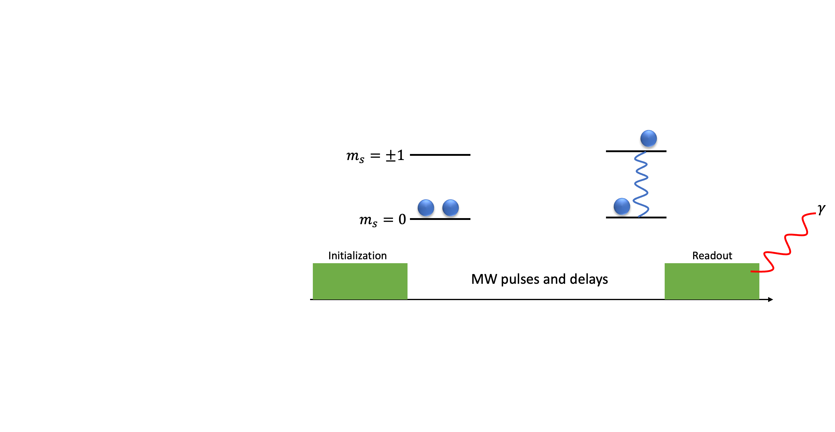
The second class of ODMR experiments we will discuss is pulsed (or time-resolved) ODMR. Figure 1 shows the basic experimental structure. The sequence begins by initializing the NV center into the state with a laser pulse. A series of microwave pulses and delays then manipulate the electronic spin state. The exact sequence of operations will depend on the specific experiment, but will be designed to create changes in populations of states or coherences between states, akin to standard pulsed EPR or NMR. At the end of this sequence, a second laser pulse allows for the readout of spin state populations.
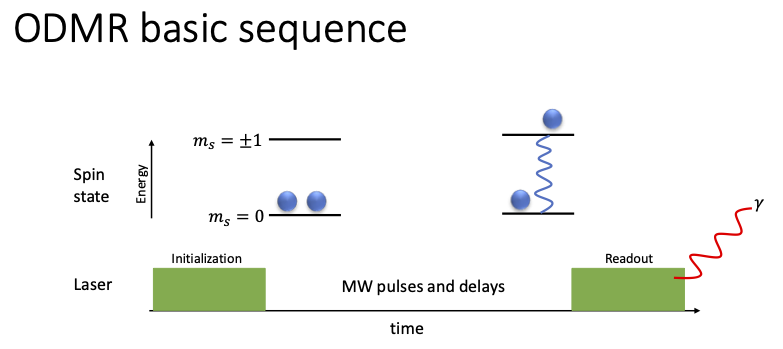 state. Microwave pulses and delays then allow for the manipulation of the spin state state, interchanging populations and/or coherences between states. A readout pulse then causes the center to fluoresce photons at 637 nm with a spin-dependent intensity. Note that here the states have the same energy for simplicity (i.e. we are at zero magnetic field), but that the same concepts apply at non-zero fields.
If we were to want information on nuclear spin states as well as electronic spin states, then we could add radiofrequency pulses during the middle block of the experiment to manipulate the nuclear spin states. In that case, we would also need to transfer any information about nuclear spins (coherences or population changes generated) back to our electronic spin state population for readout.
As one can imagine, there is a vast variety of different microwave/delay sequences that can be used for different forms of ODMR experiments. We will introduce the simplest possible sequence below, which establishes the fundamentals underlying many ODMR experiments. But we also encourage the interested reader to stay tuned for future posts on more complex ODMR experiments, and to look into the literature to learn more about the wide array of experiments in ODMR.
It may still be unclear how exactly this experimental scheme allows for the measurement of a useful magnetic resonance signal. In conventional EPR, we generally use a  followed by a
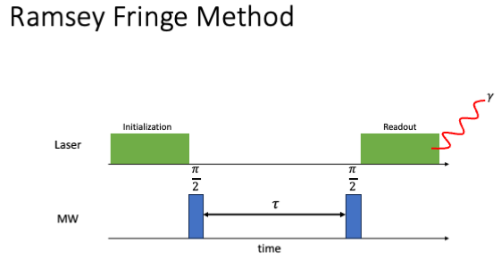
  pulse, and measure the echo observed by the rephasing of the electron spins. Meanwhile, in NMR, we can use a single pulse to rotate spins into the transverse plane. We then can measure the resulting precession about the external field to extract the time-domain signal, or free-induction decay (FID). In ODMR, we can also acquire a FID, but this requires two microwave pulses instead of one (and many repetitions). This technique is known as the Ramsey Fringe method, with a basic structure shown in Figure 2.
 , and contributes one point to the FID. By running many experiments while varying , one is able to construct the full time-domain FID.
We will walk through the phase evolution of an NV center during this sequence to better understand how it works. Like most NV ODMR experiments, the sequences begins by initializing the NV center into the state by a laser pulse. We then apply a  pulse (we will use a specific phase convention for this discussion, but other pulse phases are possible and provide similar results as long as relative phases are maintained). This pulse creates a superposition (or coherence) between our
  (
( ) and (
 ) states,
(1) 
Here we consider the case of zero field, so we can treat out NV as a two level system and say that the state is degenerate with both being in state . However, the same principles apply at non-zero fields, where one of the transitions is generally isolated to form a pseudo two level system.
Because the states and have a difference in energy  , equivalent to the zero-field splitting in our zero-field case, a phase will accumulate between the two states. Thus, the state at time will be
(2) 
At this point, we apply a  pulse to reconvert our state to populations of and . The resulting population of the state will be modulated by a term
  . Thus, the transition energy is encoded within the modulation of the population, which can be monitored via the fluorescence from the NV center.
It may be helpful to understand this phase accumulation and resulting population modulation by considering a couple different time points. If  , then our our state before the second pulse is
(3)
which we note is identical to the state immediately following the first pulse. The second pulse will then return us to our initial state of and the fluorescence intensity will be at a maximum.
On the other hand, if  , then we are in the state
(4) 
before the second pulse. The second pulse will then leave the state unchanged, so that in our final state we have only half that initial population that we initially had, and our fluorescence intensity is reduced. (Note that here we have made the assumption that we have an ensemble of NV centers, or have made the measurement many times on a single center. A single measurement on one NV center would collapse the state into either the or state, so that we could not really use phrases such as “half the population”).
To generate a time domain FID, one conducts many measurements while varying . As noted above, at each we will also have to take many measurements in order to achieve reasonable SNR in our fluorescence signal. Since each value of generates a single point in our FID (as compared to a standard pulsed NMR experiment, where the full FID is generated by a single pulse), we see that this is a time consuming process. After we have generated the FID over the course of many iterations of the experiment, processing is similar to a standard FID, where a Fourier transform of the FID will yield a one-dimensional spectrum.
As one can imagine, many more complex pulse sequences are possible in NV ODMR, including multi-dimensional experiments, but they all build on the same principles introduced above. The spin is first optically initialized into the state. Pulses then convert populations into coherences, which evolve (via delays or further microwave pulses) in time. Eventually, the coherences are returned to populations for optical readout.
A similar procedure can also measure NMR signals from nuclei coupled to the NV center (such as  N or
N or  C), but in that case a combination of microwave and radiofrequency pulses generate both electron and nuclear spin coherences, respectively. Just as above, these coherences accumulate a transition energy-dependent phase, and eventually these coherences are converted into electron spin state populations for optical readout.
You may be thinking that ODMR sounds time-consuming, and it can be! But at the same time, it offers some powerful advantages over traditional magnetic resonance techniques. For systems such as the NV, we can initialize and readout the spin state without an external field. (Note that we could have an external field, as ODMR works at non-zero fields by the same principles, and in some cases, such as detecting nuclear spins, external fields are necessary). Additionally, one can write to and read out from a single NV center, as opposed to traditional magnetic resonance experiments which measure an ensemble of spins. These properties make NV ODMR a powerful tool for a range of potential applications, from high sensitivity magnetometry to biomedical imaging to quantum information storage and processing. While some of these applications will be discussed in future posts, we also encourage the interested reader to look into the wide and exciting array of literature on ODMR and NV centers to delve deeper into the state of the art in these areas.