June 10th, 2025

NMR spectrum of ethanol

Author: Quentin Stern
Editor: Joshua Straub

In the previous post, we saw how to simulate NMR spectra for ensembles of J-coupled spins in the liquid state. In this post, we’ll use what we’ve introduced previously to simulate the ¹H NMR spectrum of ethanol. Again, we won’t need to change the script much to adapt it to this particular molecule: all the elements are already there! We’ll change one thing though: we’ll express the frequencies of the different spins as chemical shift, rather than as frequency offsets. This has the advantage to be closer to how we like to define things experimentally. The Python script can be opened, ran, and modified from this link. The MATLAB script is available here.

The spin topology of the ethanol molecule is schematized below. It’s a A₂B₃C system, in Pople’s notation. The methylene group has two equivalent ¹H spins, labelled A (spin 1 and 2); the methyl group has three equivalent ¹H spins, labelled B (spin 3, 4, and 5); finally, the alcohol group has a single ¹H spin, labelled C (spin 6). Each site A, B, and C have their own chemical shift.

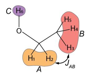
Spins A and B are coupled by a scalar coupling $J_{AB}$ . Couplings to the alcohol ¹H spin also exist. However, this proton is labile, that is, it hops on and off rapidly, much faster than the time scale of the couplings. The consequence of this is that spins A and B see an average of the effect of all the ¹H spins that spend some time on site C, and so the splittings that C should cause to A and B (and vice versa) coalesces into a single peak. This effect is often referred to as chemical exchange. We’ll certainly come back to that in future posts, as it has important consequences for NMR and can actually be used to study dynamic processes by NMR.

We first define the spin system (6 spins 1/2), the chemical shifts, and the J-coupling.

MATLAB
Python

% Spin system
SS      = [1/2 1/2 1/2 1/2 1/2 1/2];      

% Spin parameters
deltaA  = 1.2;      % Chemical shift of spins A, ppm
deltaB  = 3.7;      % Chemical shift of spins B, ppm
deltaC  = 2.6;      % Chemical shift of spin C, ppm
JAB     = 10;       % J coupling, Hz

# Spin system
SS      = [1/2, 1/2, 1/2, 1/2, 1/2, 1/2];

# Spin parameters
deltaA  = 3.7;      # Chemical shift of spins A, ppm
deltaB  = 1.2;      # Chemical shift of spins B, ppm
deltaC  = 2.6;      # Chemical shift of spin C, ppm
JAB     = 10;       # J coupling, Hz
P0      = 1e-6;     # Initial polarization, -

To convert the chemical shifts from ppm to rad.s^-1, we need to define the magnetic field at which the experiment is performed. Here, it was chosen to be $B_0 = 7$ T. We then need the gyromagnetic ratio of the ¹H spins $\gamma$ . While in the previous simulations, the center of the spectrum was always at 0 Hz, here it’s convenient to choose the center as an offset in ppm. Experimentally, this corresponds to the carrier frequency, also called the reference frequency, $\delta_\textrm{ref}$ . We also define the spectral width in ppm.

MATLAB
Python

% Experimental parameters, constants and other parameters
B0      = 7;        % Magnetic field, T
gamma   = 2.6751e8; % 1H gyromagnetic ratio, rad.s-1.T-1
deltaref= 2.5;      % Chemical shift at the center, ppm
SW      = 3.2;      % Spectral width, ppm
lb      = 0.5;      % Lorentzian line broadening, Hz  
K       = 2^12;     % Number of points in the FID, -
L       = K*4;      % Number of points in the spectrum, -

# Experimental parameters, constants and other parameters
B0      = 7;        # Magnetic field, T
gamma   = 2.6751e8; # 1H gyromagnetic ratio, rad.s-1.T-1
deltaref= 2.5;      # Chemical shift at the center, ppm
SW      = 3.2;      # Spectral width, ppm
lb      = 0.5;      # Lorentzian line broadening, Hz
K       = 4096;     # Number of points in the FID, -
L       = K*4;      # Number of points in the spectrum, -

We compute the nuclear Larmor frequency as

(1) $\begin{equation*}\omega_0 = \gamma B_0.\end{equation*}$

Technically, it should have a minus sign, but we only care about the absolute value. The offset frequencies in rad.s^-1 are then given by

(2) $\begin{equation*}\Omega_{0,k} \approx (\delta_k-\delta_\textrm{ref}) \omega_0\cdot 10^{-6}.\end{equation*}$

This equation is an approximation is the sense that $\omega_0$ should be replaced by $\omega_\textrm{TMS}$ , the nuclear Larmor frequency of tetramethylsilane, which is the reference compound for ¹H NMR, that has a chemical shift of 0 by definition. However, this approximation only brings an error of ppm of ppm.

The sampling frequency $f$ in Hz is obtained similarly as

(3) $\begin{equation*}f = \frac{\omega_0}{2\pi}S_\textrm{W}^\textrm{ppm} 10^{-6},\end{equation*}$

where $S_\textrm{W}^\textrm{ppm}$ is the spectral width in ppm.

MATLAB
Python

% Nuclear Larmor frequency, rad.s-1
omega0  = gamma*B0;

% Offset frequencies, rad.s-1
Omega0A = (deltaA-deltaref)*1e-6*omega0;
Omega0B = (deltaB-deltaref)*1e-6*omega0;
Omega0C = (deltaC-deltaref)*1e-6*omega0;

% Sampling frequency/spectral width, Hz
f       = omega0/2/pi*SW*1e-6;

# Nuclear Larmor frequency, rad.s-1
omega0  = gamma*B0;

# Offset frequencies, rad.s-1
Omega0A = (deltaA-deltaref)*1e-6*omega0;
Omega0B = (deltaB-deltaref)*1e-6*omega0;
Omega0C = (deltaC-deltaref)*1e-6*omega0;

# Sampling frequency/spectral width, Hz
f       = omega0/2/np.pi*SW*1e-6;

In principle, the thermal equilibrium density matrix (in the high temperature approximation) should be expressed as

(4) $\begin{equation*}\hat{\rho}_0=\frac{P_0}{2^{N-1}}\hat{I}_z,\end{equation*}$

where $P_0$ , $N=6$ , and $\hat{I}_z$ are the Boltzmann equilibrium spin polarization, the number of spins in the system, and the sum of the angular momentum operators along the $z$ axis for all spins, respectively. However, we drop the factor $P_0/2^{N-1}$ it for simplicity, yielding

(5) $\begin{equation*}\hat{\rho}_0=\hat{I}_z.\end{equation*}$

All the prefactor in Eq. 4 does is to scale the spectrum up and down.

MATLAB
Python

% Initial state - density matrix
rho0 = I(SS,'z');

# Initial state - density matrix
rho0 = P0*I(SS,'z')

The free evolution Hamiltonian is constructed as in the case of the coupled homonuclear spin pair in the previous post. It contains the contributions of the Zeeman and J Hamiltonians

(6) $\begin{equation*}\hat{H}_\textrm{Z} = \omega_{0,A}(\hat{I}_{1z}+\hat{I}_{2z}) + \omega_{0,B}(\hat{I}_{3z}+\hat{I}_{4z}+\hat{I}_{5z}) + \omega_{0,C}\hat{I}_{6z},\end{equation*}$

and

(7) $\begin{equation*}\hat{H}_J&=2\pi J_{AB} ( \hat{\boldsymbol{I}}_1 + \hat{\boldsymbol{I}}_2 )\cdot ( \hat{\boldsymbol{I}}_3 + \hat{\boldsymbol{I}}_4 + \hat{\boldsymbol{I}}_5).\end{equation*}$

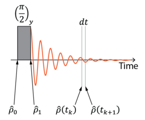
The free evolution propagator during time step $dt = 1/f$ is computed as in previous posts. The observable operator is the sum of $\hat{I}_{k+}$ over all spins.

MATLAB
Python

% Free evolution Hamiltonian
HZ = Omega0A*I(SS,1:2,'z') + Omega0B*I(SS,3:5,'z') + Omega0C*I(SS,6,'z');
HJ = 2*pi*JAB*I(SS,1:2,'dot',3:5);
H0 = HZ + HJ;

% Free evolution time propagator during dt
dt = 1/f;
U0 = expm(-1i*H0*dt);

% Observable operator
O  = I(SS,'+');

# Free evolution Hamiltonian
HZ = Omega0A*I(SS,[0,1],'z') + Omega0B*I(SS,[2,3,4],'z') + Omega0C*I(SS,5,'z')
HJ = 2*np.pi*JAB*I(SS,[0,1],'dot',[2,3,4])
H0 = HZ + HJ

# Free evolution time propagator during dt
dt = 1/f
U0 = expm(-1j*H0*dt)

# Observable operator
O  = I(SS,'+')

The part of the script doing the propagation, apodization, and Fourier transform is unchanged compared to the previous posts.

MATLAB
Python

% Empty vector to store FID
FID = zeros(1,K);

% Loop for free evolution
rhok= rho1;
for k=1:K
    % Extract expactation value
    FID(k) = trace(O*rhok);

    % Propagate during dt
    rhok = U0*rhok*U0';
end

% Apodization of the FID
T2 = 1/pi/lb;
t  = (0:K-1)*dt;
w  = exp(-t/T2);
FID= FID.*w;
FID(1) = FID(1)/2;

% Fourier transform and phasing:
spc=fftshift(fft(FID,L));

# Empty vector to store FID
FID = np.zeros(K,dtype=complex)

# Loop for free evolution
rhok = rho1
for k in range(K):
    # Extract expactation value
    FID[k] = np.trace(O@rhok)

    # Propagate during dt
    rhok = U0@rhok@U0.T.conj()

# Apodization of the FID
T2 = 1/np.pi/lb
t  = np.arange(K)*dt
w  = np.exp(-t/T2)
FID= FID*w
FID[0] = FID[0]/2

# Fourier transform and phasing
spc=np.fft.fftshift(np.fft.fft(FID,L))

In a previous post, we showed how to compute the frequency axis in Hz. To express the spectrum is ppm, we then need to convert the frequency axis using

(8) $\begin{equation*}\delta_k = \frac{2\pi\nu_k}{\omega_0}10^6 + \delta_\textrm{ref},\end{equation*}$

and we can then plot the spectrum.

MATLAB
Python

% Frequency axis, Hz
nu = (-L/2:+L/2-1)/L*f;

% Frequency axis, Hz
nuppm = 2*pi*nu/omega0*1e6 + deltaref;

% Visualization of the spectrum
figure(1), lw=1;
plot(nuppm,real(spc),'LineWidth',lw)
xlabel('Offset freq. (ppm)'), xlim([min(nuppm) max(nuppm)])
set(gca,'FontSize',12,'XDir','reverse')

# Frequency axis, Hz
nu = np.arange(-L/2,L/2)/L*f

# Frequency axis, Hz
nuppm = 2*np.pi*nu/omega0*1e6 + deltaref;

# Visualization of the spectrum
plt.figure(1)
plt.plot(nuppm,spc.real)
plt.xlabel('Offset freq. (ppm)')
plt.xlim(np.min(nuppm),np.max(nuppm))
plt.gca().invert_xaxis()
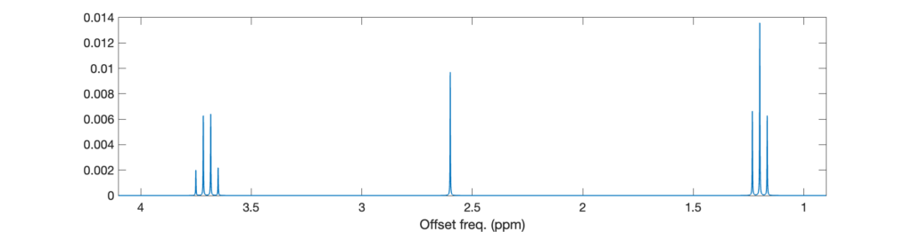
plt.show()

The spectrum features one quadruplet (spins A), one triplet (spins B), and one singlet (spin C). The signal of spins A are split into four peaks because of the interaction with the three spins B, and that of spins B is split into a three peaks because of the interaction with the two spins A. The multiplets do not feature the exact ratios 1:3:3:1 and 1:2:1 from the Pascal triangle because the coupling is not negligible compared to the frequency difference (roof effect).

Conclusion

In this post, we’ve seen how to simulate the NMR spectrum of a typical small molecule in the solution-state NMR. From here, you can start playing with the script and simulate virtually any small molecule that you want. For example, you can try to add a weakly coupled ¹³C to simulate the spectrum of the satellite peaks. That’s a suggestion, but there are thousands of interesting cases you can simulate from now on. Have fun!

To previous post:
NMR spectrum of
coupled spins

// Initialize the counter variable
$counter = 1;

// Loop from 1 to 10
while ($counter <= 10) {
// Print the current value of the counter
echo $counter . "\n";

// Increment the counter by 1
$counter++;
}
?>

1 2 3 4 5 6 7 8 9 10

#include

int main() {
// Initialize the counter variable
int counter = 1;

// Loop from 1 to 10
while (counter <= 10) {
// Print the current value of the counter
printf("%d\n", counter);

// Increment the counter by 1
counter++;
}

return 0;
}

1 2 3 4 5 6 7 8 9 10

#include

int main() {
// Initialize the counter variable
int counter = 1;

// Loop from 1 to 10
while (counter <= 10) {
// Print the current value of the counter
std::cout << counter << std::endl;

// Increment the counter by 1
counter++;
}

return 0;
}

1 2 3 4 5 6 7 8 9 10

// Initialize the counter variable
let counter = 1;

// Loop from 1 to 10
while (counter <= 10) {
// Print the current value of the counter
console.log(counter);

// Increment the counter by 1
counter++;
}

NMR spectrum of ethanol

Conclusion

Leave a Reply Cancel reply

Artist Credit:

Contact:

Website designed and developed by:

NMR spectrum of ethanol

Conclusion

Leave a Reply Cancel reply

Artist Credit:

Contact:

Website designed and developed by:

Quantum Insights