Welcome back! In the previous post, we laid out the building blocks for the simulation of NMR spectra for an ensemble of isolated spins. In this post, we will see how this can be extended to systems of multiple interacting spins. The last post was fairly long as we had a lot of concepts to introduce. This post will be rewarding as very little changes in the script will give us access to important results.
We’ll look at the example of pairs of nuclear spins, either homonuclear (e.g. two 1H spins) or heteronuclear (e.g. one 1H and one 13C spin), whether coupled or uncoupled. We still restrict ourselves to the case of liquid-state NMR, where we don’t need to take anisotropic interactions into account. The Python script can be opened, ran, and modified from this link. The MATLAB script is available here.
What do we call a spin pair here? We’re talking about an ensemble of pairs, meaning that we have many copies of the same pair. The difference between these two spins can be accounted for explicitly as they have their own states and dimensions in the Hilbert space we use to describe them. Here, we’re dealing with spins 1/2 so the Hilbert space has 4 dimensions. In the Zeeman basis, the corresponding basis states are  .
.
To simulate the NMR spectrum of these two spins, as opposed to that of a single spin, we have little to change to our script (see previous post). The first thing we need to do is to define the spin system (i.e., two spins 1/2) and the offset frequency of each spin. Because it’s a homonuclear spin system (e.g., two spins of the same type), we assume that they have the same initial polarization  .
.
% Spin system
SS      = [1/2 1/2];

% Spin parameters
Omega01 = -2*pi*20; % Offset frequency of spin 1, rad.s-1
Omega02 = +2*pi*30; % Offset frequency of spin 2, rad.s-1
P0      = 1e-6;     % Initial polarization, -
# Spin system
SS = [1/2, 1/2]
# Spin parameters
Omega01 = -2*np.pi*20;# Offset frequency of spin 1, rad.s-1
Omega02 = +2*np.pi*30;# Offset frequency of spin 2, rad.s-1
P0 = 1e-6 # Initial polarization, -We can keep the same parameters for propagation and Fourier transform that we had in the previous post.
% Parameters for propagation and Fourier transform
f       = 100;      % Sampling frequency/spectral width, Hz
lb      = 1;        % Lorentzian line broadening, Hz
K       = 2^9;      % Number of points in the FID, -
L       = K*4;      % Number of points in the spectrum, -
# Parameters for propagation and Fourier transform
f = 100 # Sampling frequency/spectral width, Hz
lb = 1 # Lorentzian line broadening, Hz
K = 512 # Number of points in the FID, -
L = K*4 # Number of points in the spectrum, -The initial density matrix of the two spins at thermal equilibrium is
(1) 
where  is the sum of the angular momentum operators of the two spins, with
  (a factor 1/2 comes up when we go from 1 to 2 spins, we’ll dedicate a post to explaining why!). Using the I function that we have introduced previously, this reads as below.
% Initial state - density matrix
rho0 = P0/2*I(SS,'z');
# Initial state - density matrix
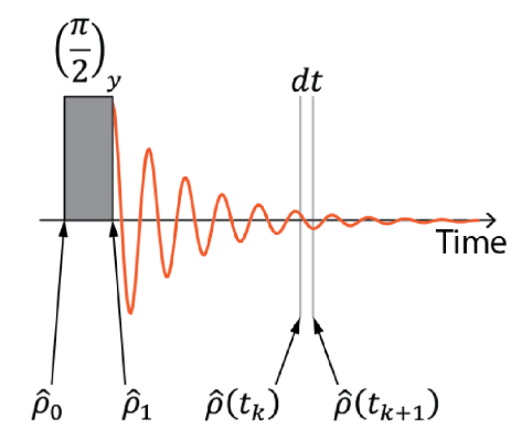
rho0 = P0/2*I(SS,'z')Assuming that the excitation pulse acts on both spins, it reads
(2) 
where  is the tip angle of the pulse, and the propagation step is the same as for the one-spin case
(3) 
% Excitation pulse propagator
Up   = expm(-1i*pi/2*I(SS,'y'));

% Excitation pulse propagation
rho1 = Up*rho0*Up';
# Excitation pulse propagator
Up = expm(-1j*np.pi/2*I(SS,'y'))
# Excitation pulse propagation
rho1 = Up@rho0@Up.T.conj()The free evolution Hamiltonian  is where we will start to see interesting differences compared to the previous case. In the case of the uncoupled spins, it only consists of the Zeeman Hamiltonian
  , which reads
(4) 
where each spin in the pair can have a different offset frequency.
% Free evolution Hamiltonian
HZ = Omega01*I(SS,1,'z') + Omega02*I(SS,2,'z');
H0 = HZ;

% Free evolution time propagator during dt
dt = 1/f;
U0 = expm(-1i*H0*dt);
# Free evolution Hamiltonian
HZ = Omega01*I(SS,0,'z') + Omega02*I(SS,1,'z')
H0 = HZ
# Free evolution time propagator during dt
dt = 1/f
U0 = expm(-1j*H0*dt)In this experiment, we are looking at two spins at the same time. Put more formally, the NMR coil is sensitive to both spins. So the observable is the sum of the observables corresponding to each spin  ,
,
(5) 
% Observable operator
O  = I(SS,'+');
# Observable operator
O = I(SS,'+')The rest of the code is exactly the same as in the single spin case.
% Propagation
% Empty vector to store FID
FID = zeros(1,K);

% Loop for free evolution
rhok= rho1;
for k=1:K
    % Extract expactation value
    FID(k) = trace(O*rhok);

    % Propagate during dt
    rhok = U0*rhok*U0';
end

% Apodization of the FID
T2 = 1/pi/lb;
t  = (0:K-1)*dt;
w  = exp(-t/T2);
FID= FID.*w;
FID(1) = FID(1)/2;

% Fourier transform and phasing
spc=fftshift(fft(FID,L));

% Frequency axis, Hz
nu = (-L/2:+L/2-1)/L*f;

% Visualization of the spectrum
figure(1)
plot(nu,real(spc),'LineWidth',lw)
xlabel('Offset freq. (Hz)'), xlim([min(nu) max(nu)])
set(gca,'FontSize',12,'XDir','reverse')
# Propagation
# Empty vector to store FID
FID = np.zeros(K,dtype=complex)
# Loop for free evolution
rhok = rho1
for k in range(K):
# Extract expactation value
FID[k] = np.trace(O@rhok)
# Propagate during dt
rhok = U0@rhok@U0.T.conj()
# Apodization of the FID
T2 = 1/np.pi/lb
t = np.arange(K)*dt
w = np.exp(-t/T2)
FID= FID*w
FID[0] = FID[0]/2
# Fourier transform and phasing
spc=np.fft.fftshift(np.fft.fft(FID,L));
# Frequency axis, Hz
nu = np.arange(-L/2,L/2)/L*f
# Visualization of the spectrum
plt.figure(1)
plt.plot(nu,spc.real)
plt.xlabel('Offset freq. (Hz)')
plt.xlim(np.min(nu),np.max(nu))
plt.gca().invert_xaxis()
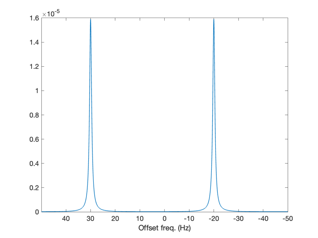
plt.show()Now, running the whole script, we get two lines, each corresponding to a different spin, as expected.
The case we have simulated in the previous section is that of non-interacting spins. Because they don’t interact, we didn’t even need to construct a 2-spin space. We could have made two distinct simulations, one per spin, and sum them up, and we would have obtained the same result. Now is where the fun starts. We will now introduce a J coupling between the two spins, so the free evolution Hamiltonian will be the sum of the Zeeman and J coupling Hamiltonians  . The full form (non truncated) of the J Hamiltonian is
(6) 
We first need to define the J coupling in the spin parameters. Annoyingly, the convention is to express the J coupling in Hz (in this example 5 Hz), while all the rest is usually expressed in rad.s-1. This is what leads to the presence of the factor  in Eq. 6.
% Spin parameters
Omega01 = -2*pi*20; % Offset frequency of spin 1, rad.s-1
Omega02 = +2*pi*30; % Offset frequency of spin 2, rad.s-1
J       = 5;        % J coupling, Hz
P0      = 1e-6;     % Initial polarization, -
# Spin parameters
Omega01 = -2*np.pi*20 # Offset frequency of spin 1, rad.s-1
Omega02 = +2*np.pi*30 # Offset frequency of spin 2, rad.s-1
J = 5 # J coupling, Hz
P0 = 1e-6 # Initial polarization, -Then, we can compute the free evolution Hamiltonian.
% Free evolution Hamiltonian
HZ = Omega01*I(SS,1,'z') + Omega02*I(SS,2,'z');
HJ = 2*pi*J*I(SS,1,'dot',2);
H0 = HZ + HJ;
# Free evolution Hamiltonian
HZ = Omega01*I(SS,0,'z') + Omega02*I(SS,1,'z')
HJ = 2*np.pi*J*I(SS,0,'dot',1)
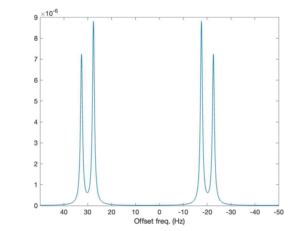
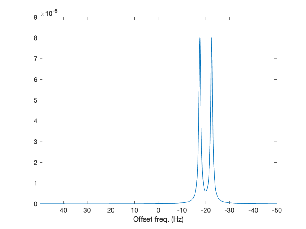
H0 = HZ + HJThat’s all there’s to change to the code to introduce the coupling between the two spins, and tadaaa, we get the spectrum below! Now, the peak corresponding to each spin is split by the J coupling, into two lines whose intensities are approximately half that of the original line. Why not exactly one half? Because the J coupling is not negligible compared to the frequency difference between the spins (5 Hz compared to 40 Hz), the spins are not weakly coupled and their spectrum features the roof effect. We’ll come back to that in a future post!
Another interesting case is that of a heteronuclear spin pairs, like for example a 1H and a 13C spins. There are a few things that we need to adapt. First, the two spins will have different initial polarization. That will not play a big role here, but might for some other experiments. Second, the J Hamiltonian is usually expressed in the truncated form (see below). Last, in a typical experiment, we only look at single spin species at a time, either 1H and a 13C, which will affect the way we define the pulse propagator and the observable.
We start by introducing a different initial polarization for the two spins. In the high temperature approximation, the Boltzmann polarization is proportional to the gyromagnetic ratio, which is 4 times larger for 1H than for 13C spins. Setting spin 1 and 2 as the 1H and 13C spins, respectively, we can write their polarizations as below, to respect the polarization ratio.
% Spin system
SS      = [1/2 1/2];

% Spin parameters
Omega01 = -2*pi*20; % Offset frequency of spin 1, rad.s-1
Omega02 = +2*pi*30; % Offset frequency of spin 2, rad.s-1
J       = 5;        % J coupling, Hz
P01     = 4e-6;     % Initial polarization of spin 1, -
P02     = 1e-6;     % Initial polarization of spin 2, -
# Spin system
SS = [1/2, 1/2]
# Spin parameters
Omega01 = -2*np.pi*20 # Offset frequency of spin 1, rad.s-1
Omega02 = +2*np.pi*30 # Offset frequency of spin 2, rad.s-1
J = 5 # J coupling, Hz
P01 = 4e-6 # Initial polarization of spin 1, -
P02 = 1e-6 # Initial polarization of spin 2, -The initial density matrix of the two spins at thermal equilibrium is then
(7) 
% Initial state - density matrix
rho0 = P02/2*I(SS,1,'z') + P02/2*I(SS,2,'z');
# Initial state - density matrix
rho0 = P01/2*I(SS,0,'z') + P02/2*I(SS,1,'z')As we mentioned, we are only looking at a single spin species at a time, either 1H and a 13C. Here, we choose to look at spin 1, i.e., the 1H spin, and we only pulse on the 1H spin. The pulse propagator therefore reads
(8) 
The reason why the pulse on one spin does not affect the other spin comes from the fact that pulses have a limited bandwidth (typ. in the tens of kHz), while the separation frequency difference is on the order of hundreds of MHz.
% Excitation pulse propagator
Up   = expm(-1i*pi/2*I(SS,1,'y'));

% Excitation pulse propagation
rho1 = Up*rho0*Up';
# Excitation pulse propagator
Up = expm(-1j*np.pi/2*I(SS,0,'y'))
# Excitation pulse propagation
rho1 = Up@rho0@Up.T.conj()For the hetereonuclear spin case, the truncated J Hamiltonian is usually used, where we remove terms that don’t commute with the Zeeman Hamitlonian,
(9) 
We could keep the full form as expressed in Eq. 6. This would leave the simulation unchanged.
% Free evolution Hamiltonian
HZ = Omega01*I(SS,1,'z') + Omega02*I(SS,2,'z');
HJ = 2*pi*J*I(SS,1,'z',2,'z');
H0 = HZ + HJ;
# Free evolution Hamiltonian
HZ = Omega01*I(SS,0,'z') + Omega02*I(SS,1,'z')
HJ = 2*np.pi*J*I(SS,0,'z',1,'z')
H0 = HZ + HJThe last thing we need to adapt is that the NMR coil is only sensitive to 1H spins so the observable is
(10) 
% Observable operator
O  = I(SS,1,'+');
# Observable operator
O = I(SS,0,'+')The rest of the script is unchanged. The resulting spectrum is below. It features one doublet corresponding to the 1H spin, and the splitting comes from the 13C spin, which doesn’t appear in the spectrum. The two lines in the doublet have equal intensity because the spins are weakly coupled, that is, the doublet doesn’t feature the roof effect.
In this post, we’ve seen how to simulate the NMR spectrum of coupled spins in the liquid state. With that, we have expanded our toolbox to a point where we can already cover a large range of important experiments simply by changing the free evolution Hamiltonian and the sequence of events. For example, this formalism can be used to describe polarization transfers (e.g., using the INEPT sequence) or quantum gates. In the next, the (fermented) cherry on the top of the cake will be to simulate the 1H spectrum of ethanol, and again, we’ll have very little changes to bring to the script.
And then what? Many experiments can only be described adequately if relaxation processes are included (e.g., continuous wave saturation in the case of dynamic nuclear polarization). Plus, we’ve only covered the case of liquid-state NMR, where anisotropic interaction are averaged out by rapid tumbling. To describe NMR in the solid state, we need to include powder averaging in our simulations. We’ll cover all this in upcoming posts!