Hi reader! This post is the first of hopefully a long series, where we will show how to simulate magnetic resonance experiments, starting from the basics (e.g., the liquid-state 1D NMR spectrum of a simple spin system), and building up to more complicated topics like multidimensional experiments or quantum gates.
The aim of these posts is not to obtain the most performant computation. If that’s what you’re searching for, you’d rather use simulation packages that have been well optimized by clever people. Our aim here is to learn how things work by coding them. For this reason, we don’t want to use a lot of external functions that would hide away some parts of the code. In all the posts that I will write, I will make use of a single predefined function, to compute angular momentum operators. Why? Because even with only two spins, you already have a set of 16 operators, and as you add more spins, the list gets very long. Yet, there’s not much to learn in this lengthy and repetitive process of constructing the operators. In fact, this approach is exactly what I use for my own research. I’m not making up something different for the purpose of these posts.
This first post is about how angular momentum operators are generated in MATLAB and Python. We will start by showing how single-spin operators are generated from scratch for arbitrary values of the the spin number  . Then, we will use the Kronecker product to compute operators in systems containing multiple spins. Once we’ve learnt how to code the operators from scratch, we will see how to compute them using the function that I wrote. Finally, we will show some example Hamiltonians that we can compute using this function (e.g., for the five 1H spins of ethanol in the liquid state).
Note that we will omit  in the expression of the operators because all Hamiltonians will be expressed in terms of rad.s-1. The full Python script presented in this post is available here (it can be run and modified directly in your browser, provided you have a Google account) and the full MATLAB script is available here.
For a single spin 1/2, the three Cartesian operators expressed in terms of Pauli matrices in the Zeeman basis read
(1) 
where  are the Pauli matrices, with the identity
(2) 
For a single spin 1, they read
(3) 
with the identity
(4) 
The dimension of the matrix representing the angular momentum operator for a spin  is
is  , yielding
  and
and  for spins 1/2 and 1, respectively. The expressions for cases with
  are given below.
For any spin number , there are  possible projections of the angular momentum
  , with
 ![m\in[-I,-I+1,..., +I-1, +I]](https://quantum-resonance.org/wp-content/ql-cache/quicklatex.com-238df0bbd5b3e29eff674b2c2c06836e_l3.png "Rendered by QuickLaTeX.com") . Writing the Zeeman states as
. Writing the Zeeman states as  , the matrix elements of the angular momentum operators read

where  is the Kronecker delta function

The elements of the corresponding identity matrix are given by

It is useful to define shift operators as
(5) 
In the case of  , the shift operators read
(6) 
The code snippet below shows how operators for spin 1/2 and 1 are generated programatically.
% Definition of the angular momentum operators for I = 1/2
Ix2x2   = [0  +1;+1  0]/2;
Iy2x2   = [0  -1;+1  0]*1i/2;
Iz2x2   = [+1  0; 0 -1]/2;
E2x2    = eye(2);
Ip2x2   = Ix2x2 + 1i*Iy2x2;
Im2x2   = Ix2x2 - 1i*Iy2x2;

% Definition of the angular momentum operators for I = 1
Ix3x3   = [0  +1 0;+1  0 +1; 0  +1  0]/sqrt(2);
Iy3x3   = [0  -1 0;-1  0 +1; 0  +1  0]*1i/sqrt(2);
Iz3x3   = [+1  0 0; 0  0  0; 0  0  -1];
E3x3    = eye(3);
Ip3x3   = Ix3x3 + 1i*Iy3x3;
Im3x3   = Ix3x3 - 1i*Iy3x3;
# Required package for numerical calculations
import numpy as np
# Definition of the angular momentum operators for I = 1/2
Ix2x2 = np.array([[0, +1/2],[ +1/2, 0]])
Iy2x2 = np.array([[0, -1j/2],[+1j/2, 0]])
Iz2x2 = np.array([[+1/2, 0],[0, -1/2]])
E2x2 = np.eye(2)
Ip2x2 = Ix2x2 + 1j*Iy2x2
Im2x2 = Ix2x2 - 1j*Iy2x2
# Definition of the angular momentum operators for I = 1
Ix3x3 = np.array([[ 0, +1, 0],[+1, 0, +1],[0, +1, 0]])/np.sqrt(2)
Iy3x3 = np.array([[ 0, -1, 0],[-1, 0, +1],[0, +1, 0]])*1j/np.sqrt(2)
Iz3x3 = np.array([[+1, 0, 0],[ 0, 0, 0],[0, 0, -1]])
E3x3 = np.eye(3)
Ip3x3 = Ix3x3 + 1j*Iy3x3
Im3x3 = Ix3x3 - 1j*Iy3x3To represent multiple spins in the same system, we need to take Kronecker products of the individual spin operators. If the system contains  spins with spin numbers
  , the operator
  of spin
  with
with  represented in the space of the spins is given by
(7) 
where the operators  are defined in the subspace of the
  spin (i.e., one of the single-spin operators that we have defined in the previous section) as
(8) 
and have dimensions of  . What Eq. 7 tells us is that to obtain an angular momentum operator of spin in the larger space of the spins, we need to take the Kronecker product over all spins, using the identity operator for each spin in its own subspace, except for , where we use the operator of interest in its own subspace (e.g.,
  or
or  ).
).
The Kronecker product is an operation that takes two matrices with dimensions  and
and  and returns a matrix with dimension
  . For an example, for two matrices of dimension , the Kronecker product is

This example calculation can easily be extended to higher dimensions.
For example, if we want to compute the  angular momentum for a pair of spins 1/2, we have
(9) 
for the first spin, and
(10) 
for the second. We only show this simple case because, as you have probably noticed, the dimensions rapidly increase when we add more spins, and the matrices become quite large to write out!
It is sometimes useful to define operators that correspond to the sum of the operators of all spins for a certain 
(11) 
For example, the sum of the angular momentum operators in a system consisting of a pair of spins 1/2 is
(12) 
The code snippet below shows how the Cartesian operators for a system of two spins 1/2 and one spin 1 are constructed, using the single-spin operators defined in the previous code snippet.
% Definition of the angular momentum operators
% of individual spins in a system of 2 spins 1/2
% and 1 spins 1
I1x     = kron(kron(Ix2x2,E2x2),E3x3);
I1y     = kron(kron(Iy2x2,E2x2),E3x3);
I1z     = kron(kron(Iz2x2,E2x2),E3x3);

I2x     = kron(kron(E2x2,Ix2x2),E3x3);
I2y     = kron(kron(E2x2,Iy2x2),E3x3);
I2z     = kron(kron(E2x2,Iz2x2),E3x3);

I3x     = kron(kron(E2x2,E2x2),Ix3x3);
I3y     = kron(kron(E2x2,E2x2),Iy3x3);
I3z     = kron(kron(E2x2,E2x2),Iz3x3);

% Sum of the angular mommentum operators
Ix      = I1x + I2x + I3x;
Iy      = I1y + I2y + I3y;
Iz      = I1z + I2z + I3z;
# Definition of the angular momentum operators
# of individual spins in a system of 2 spins 1/2
# and 1 spin 1
I1x = np.kron(np.kron(Ix2x2, E2x2),E2x2)
I1y = np.kron(np.kron(Iy2x2, E2x2),E2x2)
I1z = np.kron(np.kron(Iz2x2, E2x2),E2x2)
I2x = np.kron(np.kron(E2x2, Ix2x2),E2x2)
I2y = np.kron(np.kron(E2x2, Iy2x2),E2x2)
I2z = np.kron(np.kron(E2x2, Iz2x2),E2x2)
I3x = np.kron(np.kron(E2x2, E2x2),Ix2x2)
I3y = np.kron(np.kron(E2x2, E2x2),Iy2x2)
I3z = np.kron(np.kron(E2x2, E2x2),Iz2x2)
# Sum of the angular mommentum operators
Ix = I1x + I2x + I3x
Iy = I1y + I2y + I3y
Iz = I1z + I2z + I3zNow we move on to the function I that I promised in the introduction of this post. This function generates angular momentum operators for any spin system using a minimum of two arguments. The first argument is always a list containing the spin number of each spin in the system (e.g.,  ). Depending on the number of remaining arguments, the function will output different types of operators
 or
or  .
. or
or  .
.As mentioned above, the function I can generate single-spin operators with either 2 or 3 arguments.
 : must be a string containing one of the elements
  , and the output is the sum of all operators corresponding to , as defined in Eq. 11.
 : the second argument is the index or the list of indices corresponding to the spins for which the operator is to be computed. The third argument is a string containing one of the
  . If a list is given as second input, then the output is the angular momentum operator for summed over all spins in the list .
The code snippet below shows examples.
% Definition of the spin system
SS  = [1/2 1/2 1];

% Definition of the angular momentum operators
% of individual spins in a system of 3 spins 1/2
I1x = I(SS,1,'x');
I1y = I(SS,1,'y');
I1z = I(SS,1,'z');
I1p = I(SS,1,'+');
I1m = I(SS,1,'-');

I2x = I(SS,2,'x');
I2y = I(SS,2,'y');
I2z = I(SS,2,'z');
I2p = I(SS,2,'+');
I2m = I(SS,2,'-');

I3x = I(SS,3,'x');
I3y = I(SS,3,'y');
I3z = I(SS,3,'z');
I3p = I(SS,3,'+');
I3m = I(SS,3,'-');
# Definition of the spin system
SS = [1/2, 1/2, 1]
# Definition of the angular momentum operators
# of individual spins in a system of 3 spins 1/2
I1x = I(SS, 0, 'x')
I1y = I(SS, 0, 'y')
I1z = I(SS, 0, 'z')
I1p = I(SS, 0, '+')
I1m = I(SS, 0, '-')
I2x = I(SS, 1, 'x')
I2y = I(SS, 1, 'y')
I2z = I(SS, 1, 'z')
I2p = I(SS, 1, '+')
I2m = I(SS, 1, '-')
I3x = I(SS, 2, 'x')
I3y = I(SS, 2, 'y')
I3z = I(SS, 2, 'z')
I3p = I(SS, 2, '+')
I3m = I(SS, 2, '-')The sum of the angular momentum operators can be computed in three different ways. First, using the function with only two arguments; second, using three arguments where the second argument is the list of all spin indices; last, writing the sum explicitly. The code snippet below shows these three cases for a system of three spins.
Ix  = I(SS, 'x');
Iy  = I(SS, 'y');
Iz  = I(SS, 'z');
Ip  = I(SS, '+');
Im  = I(SS, '-');

Ix  = I(SS, 1:3, 'x');
Iy  = I(SS, 1:3, 'y');
Iz  = I(SS, 1:3, 'z');
Ip  = I(SS, 1:3, '+');
Im  = I(SS, 1:3, '-');

Ix  = I(SS,1,'x') + I(SS,2,'x') + I(SS,3,'x');
Iy  = I(SS,1,'y') + I(SS,2,'y') + I(SS,3,'y');
Iz  = I(SS,1,'z') + I(SS,2,'z') + I(SS,3,'z');
Ip  = I(SS,1,'+') + I(SS,2,'+') + I(SS,3,'+');
Im  = I(SS,1,'-') + I(SS,2,'-') + I(SS,3,'-');
Ix = I(SS, 'x')
Iy = I(SS, 'y')
Iz = I(SS, 'z')
Ip = I(SS, '+')
Im = I(SS, '-')
Ix = I(SS, [0, 1, 2], 'x')
Iy = I(SS, [0, 1, 2], 'y')
Iz = I(SS, [0, 1, 2], 'z')
Ip = I(SS, [0, 1, 2], '+')
Im = I(SS, [0, 1, 2], '-')
Ix = I(SS,0,'x') + I(SS,1,'x') + I(SS,2,'x')
Iy = I(SS,0,'y') + I(SS,1,'y') + I(SS,2,'y')
Iz = I(SS,0,'z') + I(SS,1,'z') + I(SS,2,'z')
Ip = I(SS,0,'+') + I(SS,1,'+') + I(SS,2,'+')
Im = I(SS,0,'-') + I(SS,1,'-') + I(SS,2,'-')When more than 3 arguments are provided to the function I, it outputs mutliple-spin operators, also called product operators. These operators are nothing more than the product of two or more of the operators defined above, and so can be calculated by matrix multiplication. However, in the interest of making the scripts as compact and readable as possible, I found it useful to make the function directly output products of operators. The first argument is as always the list of spin numbers. Then, there are two options
 or
or  and so on: The arguments following SS come in pairs. For each pair, the first and second of each pair are the index of the spin (or list of indices)
  and the value of defined as a string, respectively. If all contain a single element, the resulting operator is the product of the operators corresponding to each pair or arguments. If some of the content a list, the resulting operator is the sum of combinations of spins of each list.
 computes the sum of the dot products between the spins listed in
  and those listed in
  (see details below).
Below is a list of possible uses of this option for a 2-spin and a 3-spin operators in the same spin system as above. In both cases, two ways to compute the same operators are shown.
% Definition of the spin system
SS  = [1/2 1/2 1];

% Example of 2-spin operator
I1x2z   = I(SS,1,'x')*I(SS,2,'z');
I1x2z   = I(SS,1,'x',2,'z');

% Example of 3-spin operator
I1z2z3z = I(SS,1,'z')*I(SS,2,'z')*I(SS,3,'z');
I1z2z3z = I(SS,1,'z',2,'z',3,'z');

% Example of sum of 2-spin operators for an A2X system (where 1 and 2 are A and 3 is X)
IAxXz   = I(SS,1,'x')*I(SS,3,'z') + I(SS,2,'x')*I(SS,3,'z');
IAxXz   = I(SS,[1 2],'x',3,'z');
# Definition of the spin system
SS = [1/2, 1/2, 1]
# Example of 2-spin operator
I1x2z = I(SS,0,'x')@I(SS,1,'z')
I1x2z = I(SS,0,'x',1,'z')
# Example of 3-spin operator
I1z2z3z = I(SS,0,'z')@I(SS,1,'z')@I(SS,2,'z')
I1z2z3z = I(SS,0,'z',1,'z',2,'z')
# Example of sum of 2-spin operators for an A2X system (where 1 and 2 are A and 3 is X)
IAxXz = I(SS,0,'x')@I(SS,2,'z') + I(SS,1,'x')@I(SS,2,'z')
IAxXz = I(SS,0,'x',2,'z') + I(SS,1,'x',2,'z')
IAxXz = I(SS,[0, 1],'x',2,'z')The dot product between two spins and can be written in several forms
(13) 
Two of these forms can be computed using the I function, the most compact being the one corresponding to the left hand side of Eq. 13. In this case, the second, third, and fourth arguments are the index of the first spin, the string ‘dot’, and the index of the second spin, respectively. The function also supports lists of indices in the second and fourth arguments, which can be useful when dealing with equivalent spins, as in the example of the next section.
The code snippet below shows how to compute the dot product using different approaches, and demonstrates the compactness of using the ‘dot’ option of I. It is applied to two cases: the first is the dot product of spin 1 and spin 2; the second is the dot product of spins 1 and 2 with spin 3, in other words, since the dot product is distributive, the sum of the dot products of spin 1 and spin 2 and of spin 2 and spin 3.
% Scalar product operator ot spin 1 with spin 2
I1dot2  = I(SS,1,'x')*I(SS,2,'x') + I(SS,1,'y')*I(SS,2,'y') + I(SS,1,'z')*I(SS,2,'z');
I1dot2  = I(SS,1,'dot',2);

% Scalar product operator ot spin 1 and 2 with spin 3
I12dot3 = I(SS,1,'x')*I(SS,3,'x') + I(SS,1,'y')*I(SS,3,'y') + I(SS,1,'z')*I(SS,3,'z')+ ...
          I(SS,2,'x')*I(SS,3,'x') + I(SS,2,'y')*I(SS,3,'y') + I(SS,2,'z')*I(SS,3,'z');
I12dot3 = I(SS,1,'dot',3) + I(SS,2,'dot',3);
I12dot3 = I(SS,[1 2],'dot',3);
# Dot product operator of spin 1 with spin 2
I1dot2 = I(SS,0,'x')@I(SS,1,'x') + I(SS,0,'y')@I(SS,1,'y') + I(SS,0,'z')@I(SS,1,'z')
I1dot2 = I(SS,0,'x',1,'x') + I(SS,0,'y',1,'y') + I(SS,0,'z',1,'z')
I1dot2 = I(SS,0,'dot',1)
# Dot product operator ot spin 1 and 2 with spin 3
I12dot3 = I(SS,0,'x')@I(SS,2,'x') + I(SS,0,'y')@I(SS,2,'y') + I(SS,0,'z')@I(SS,2,'z') \
+ I(SS,1,'x')@I(SS,2,'x') + I(SS,1,'y')@I(SS,2,'y') + I(SS,1,'z')@I(SS,2,'z')
I12dot3 = I(SS,0,'x',2,'x') + I(SS,0,'y',2,'y') + I(SS,0,'z',2,'z') \
+ I(SS,1,'x',2,'x') + I(SS,1,'y',2,'y') + I(SS,1,'z',2,'z')
I12dot3 = I(SS,0,'dot',2) + I(SS,1,'dot',2)
I12dot3 = I(SS,[0,1],'dot',2)The function I comes in handy when dealing with large numbers of spins and their couplings. Take for example the five 1H spins in the ethyl chain of the molecule of ethanol in the liquid state.
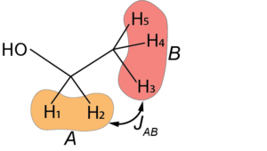
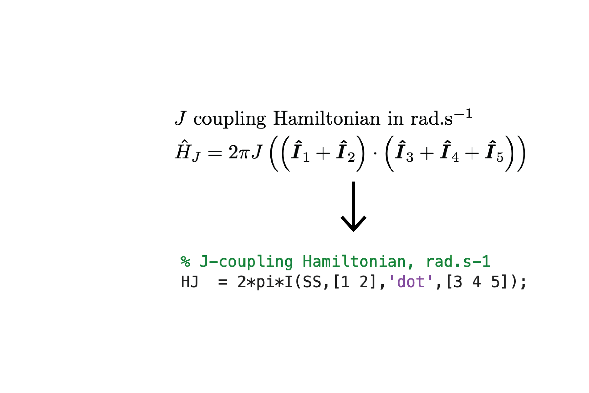
The two methylene 1H spins (labelled A, spins 1 and 2) are J coupled with the three methyl 1H spins (labelled B, spins 3, 4, and 5). The J-Hamiltonian therefore reads
(14) 
where the dot products can be expanded in Cartesian coordinates, using Eq. 13, and  Hz. This Hamiltonian would be quite long to write if we were to compute each operator manually and assemble them to make all the dot products. Using the I function, it takes the form shown in the snippet below.
% Spin sytem - 5 spins 1/2
SS  = [1/2 1/2 1/2 1/2 1/2];

% J coupling, Hz
JAB = 10;

% J-coupling Hamitlonian, rad.s-1
HJ  = 2*pi*JAB*I(SS,[1 2],'dot',[3 4 5]);
# Spin sytem - 5 spins 1/2
SS = [1/2, 1/2, 1/2, 1/2, 1/2]
# J coupling, Hz
JAB = 10
# J-coupling Hamitlonian, rad.s-1
HJ = 2*np.pi*JAB*I(SS,[0, 1],'dot',[2, 3, 4])Another example is the dipolar coupling Hamiltonian, which can be written in different forms
(15) 
The code snippet below shows all three forms.
% Spin sytem - 2 spins 1/2
SS  = [1/2, 1/2];

% Dipolar coupling, rad.s-1
D0  = 2*pi*10e3;

% Dipolar Hamitlonian, rad.s-1
HD  = D0*(3*I(SS,1,'z',2,'z') - I(SS,1,'dot',2));
HD  = D0*(2*I(SS,1,'z',2,'z') - 1/2*(I(SS,1,'+',2,'-') + I(SS,1,'-',2,'+')));
HD  = D0*(2*I(SS,1,'z',2,'z') - (I(SS,1,'x',2,'x') + I(SS,1,'y',2,'y')));
# Homonuclear dipolar coupling Hamiltonian
# Spin sytem - 2 spins 1/2
SS = [1/2, 1/2]
# Dipolar coupling, rad.s-1
D0 = 2*np.pi*10e3
# Dipolar Hamitlonian, rad.s-1
HD = D0*(3*I(SS,0,'z',1,'z') - I(SS,0,'dot',1))
HD = D0*(2*I(SS,0,'z',1,'z') - 1/2*(I(SS,0,'+',1,'-') + I(SS,0,'-',1,'+')))
HD = D0*(2*I(SS,0,'z',1,'z') - (I(SS,0,'x',1,'x') + I(SS,0,'y',1,'y')))This post was perhaps not the most exciting. Very technical and not a lot of “concrete” results. But it gives a good basis to move on to spin physics simulations, where we will regularly make use of the I function. The next post will be on simulating the NMR spectrum of simple spin systems. Stay tuned!