November 12th, 2025

Time evolution of the density matrix

Author: Quentin Stern
Editor: Joshua Straub

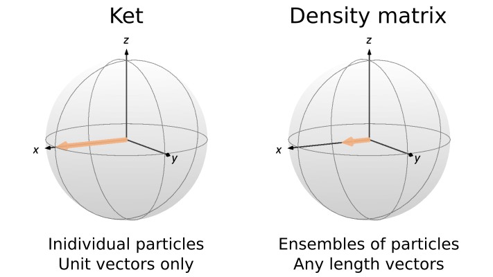
Welcome back! In the first post of this series, we’ve defined the density matrix and in the second one, we saw how to use it to extract expectation values. In this post, we will see how the density matrix evolves in time. We will first derive the Liouville-Von Neumann equation, which is the density matrix equivalent to the time-dependent Schrödinger equation, and show how it can be used to find analytical solutions for the evolution of spin systems. We will then search for the solution to the Liouville-Von Neumann equation in terms of the time propagator. Finally, we will use this solution and numerical simulation to describe the evolution of a simple spin system both with time-independent and time-dependent Hamiltonians. The MATLAB scripts can be downloaded from here. The Python scripts can be accessed and ran from here.

Liouville-Von Neumann equation

We already know how the ket describing a system evolves in time (see this post). That’s defined by the time-dependent Schrödinger equation

(1) $\begin{equation*}\frac{d}{dt}\ket{\psi(t)}=-i\hat{H}(t)\ket{\psi(t)},\end{equation*}$

where $\hat{H}(t)$ is the Hamiltonian acting on the system at time $t$ , expressed in units of angular frequency (that is, setting $\hbar = 1$ ). The evolution of the density matrix is obtained by plugging Eq. 1 into the definition of the density matrix $\hat{\rho} = \overline{\ket{\psi}\bra{\psi}}$ ,

(2) $\begin{equation*}\frac{d}{dt}\hat{\rho}(t)=-i[\hat{H}(t),\hat{\rho}(t)],\end{equation*}$

where $[\hat{A},\hat{B}] = \hat{A}\hat{B}-\hat{B}\hat{A}$ is the commutator of operators $\hat{A}$ and $\hat{B}$ (the commutation relations of the angular momentum operators are given below). Eq. 2 is called the Liouville-Von Neumann (LvN) equation.

Calculation details

The LvN equation gives us insight into the evolution of quantum mechanical systems. Indeed, it shows that the density matrix (and hence, the system) will only evolve if there exist terms in the Hamiltonian that do not commute with the density operator.

For example, if a spin is aligned with a magnetic field $B_0$ (that we choose to be along $z$ ), the density matrix and the Hamiltonian can be expressed as $\hat{\rho} = \hat{I}_z$ and $\hat{H}_0 = \omega_0\hat{I}_z$ , respectively, where $\omega_0$ is the Larmor frequency of the spin. Because $[\hat{H},\hat{\rho}]=\omega_0[\hat{I}_z,\hat{I}_z]=0$ , the LvN equation tells us that system will not evolve (that is, it will remain in the state $\hat{\rho} = \hat{I}_z$ ). To the contrary, if the system is a spin aligned perpendicular to $B_0$ , say along the $x$ axis, then we can write $\hat{\rho} = \hat{I}_x$ . In this case, the commutator of the Hamiltonian and the density matrix is non zero $[\hat{H},\hat{\rho}]=\omega_0[\hat{I}_z,\hat{I}_x]=i\omega_0\hat{I}_y$ . According to Eq. 2, $\hat{I}_z$ takes $\hat{I}_x$ into $\hat{I}_y$ .

This discussion leads us to the important conclusion that all the conditions below are equivalent

$[\hat{H},\hat{\rho}]=0$
$\hat{H}$ and $\hat{\rho}$ have identical eigenbases
$\ket{\psi}$ is an eigenstate of $\hat{H}$
$\hat{\rho}$ and $\ket{\psi}$ are stationary

while all the following are equivalent

$[\hat{H},\hat{\rho}]\ne 0$
$\hat{H}$ and $\hat{\rho}$ have distinct eigenbases
$\ket{\psi}$ is not an eigenstate of $\hat{H}$
$\hat{\rho}$ and $\ket{\psi}$ are not stationary

LvN equation and cyclic commutation

A situation that we will often encounter is that operators “turn into one another” in a closed loop. This is the case for the three angular momentum operators which satisfy the commutation relations,

(3) $\begin{equation*}\begin{split} [\hat{I}_x,\hat{I}_y] & = i\hat{I}_z \\ [\hat{I}_y,\hat{I}_z] & = i\hat{I}_x \\ [\hat{I}_z,\hat{I}_x] & = i\hat{I}_y,\end{split} \end{equation*}$

which can be summarized as

(4) $\begin{equation*}[\hat{I}_x,\hat{I}_y] = i\hat{I}_z \circlearrowleft .\end{equation*}$

This set of commutation relations is called cyclic commutation because the three operators and their commutators form a closed loop. Together, the LvN equation and the cyclic commutation of the angular momentum operators tell us that $\hat{I}_x$ turns $\hat{I}_y$ into $\hat{I}_z$ , $\hat{I}_y$ turns $\hat{I}_z$ into $\hat{I}_x$ , and $\hat{I}_z$ turns $\hat{I}_x$ into $\hat{I}_y$ .

One might recognize that this corresponds to a set of differential equations defining rotations. For example, for a spin along the $x$ axis at time $t=0$ (i.e., $\hat{\rho}(0) = \hat{I}_x$ ), a magnetic field along the $z$ axis ( $\hat{H}_0 = \omega_0\hat{I}_z$ ) will rotate the spin about the $z$ axis, yielding the solution

(5) $\begin{equation*}\hat{\rho}(t) = \cos(\omega_0 t)\hat{I}_x + \sin(\omega_0 t)\hat{I}_y,\end{equation*}$

that we sometimes like to write as

(6) $\begin{equation*}\hat{\rho}(0) \xrightarrow{\omega_0t\hat{I}_z}\cos(\omega_0 t)\hat{I}_x + \sin(\omega_0 t)\hat{I}_y,\end{equation*}$

which means that $\hat{H}_0 = \omega_0\hat{I}_z$ acts on $\hat{\rho}(0)$ for a time $t$ . It can easily be verified that Eq. 5 is a solution to the LvN equation with initial condition $\hat{\rho}(0) = \hat{I}_x$ .

Proof

Using Eq. XXX from the previous post (link XXX), we find that the expectation values of the angular momentum operators along the Cartesian coordinates are

(7) $\begin{equation*}\begin{split}\braket{\hat{I}_x(t)} & = \text{Tr}\left(\hat{I}_x\hat{\rho}(t)\right)= \frac{1}{2}\cos \left(\omega_0 t\right) \\\braket{\hat{I}_y(t)} & = \text{Tr}\left(\hat{I}_y\hat{\rho}(t)\right)= \frac{1}{2}\sin \left(\omega_0 t\right)\\\braket{\hat{I}_x(t)} & = \text{Tr}\left(\hat{I}_z\hat{\rho}(t)\right)= 0.\end{split}\end{equation*}$

Calculation details

We obtained this result using the ket formalism in this post. Here, we have found that the same result is obtained using the density matrix formalism, but perhaps in an easier way, which requires less calculations (and don’t we love that?).

We have shown how the cyclic commutation relations help us track the evolution of the three Cartesian angular momentum operators in time. But it’s in fact much more general. Indeed, for any set of three operators $\hat{A}$ , $\hat{B}$ , and $\hat{C}$ fulfilling the cycling commutation relation

(8) $\begin{equation*}[\hat{A},\hat{B}] = i\hat{C} \circlearrowleft ,\end{equation*}$

we have that

(9) $\begin{equation*}\begin{split}\hat{A} & \xrightarrow{\omega t\hat{B}}\cos(\omega t)\hat{A} + \sin(\omega t)\hat{C} \\\hat{B} & \xrightarrow{\omega t\hat{C}}\cos(\omega t)\hat{B} + \sin(\omega t)\hat{A} \\\hat{C} & \xrightarrow{\omega t\hat{A}}\cos(\omega t)\hat{C} + \sin(\omega t)\hat{B} ,\end{split}\end{equation*}$

and, because $[\hat{A},\hat{B}]=-[\hat{B},\hat{A}]$ ,

(10) $\begin{equation*}\begin{split}\hat{B} & \xrightarrow{\omega t\hat{A}}\cos(\omega t)\hat{B} - \sin(\omega t)\hat{C} \\\hat{C} & \xrightarrow{\omega t\hat{B}}\cos(\omega t)\hat{C} - \sin(\omega t)\hat{A} \\\hat{A} & \xrightarrow{\omega t\hat{C}}\cos(\omega t)\hat{A} - \sin(\omega t)\hat{B} .\end{split}\end{equation*}$

So far, we have seen one example of cyclic commutation relation, that of the Cartesian angular momentum operator of a single spin. In future posts, we will see that coupled spins have multiple spin operators (e.g. $2\hat{I}_{1z}\hat{I}_{2z}$ ) with their own cyclic commutation relations. The results we have just obtained (Eqs. 9 and 10) will be at the core of how we will track analytically the evolution of quantum mechanical systems in time.

Solution to the LvN equation

Cyclic commutations is one way to use the LvN equation. Another way to use it is by solving it. That’s what we do in this section. As we have shown (see this post), for a time-independent Hamiltonian, the time-dependent Schrödinger equation has a convenient solution

(11) $\begin{equation*}\ket{\psi(t)} = \hat{U}(t)\ket{\psi(0)},\end{equation*}$

expressed in terms of the propagator

(12) $\begin{equation*}\hat{U}(t) = \exp{\left(-i\hat{H}t\right)},\end{equation*}$

where it is assumed, again, that the Hamiltonian is expressed in rad.s^-1, and not in Joules. This equation has an equivalent in terms of the density matrix,

(13) $\begin{equation*}\hat{\rho}(t)=\hat{U}(t)\hat{\rho}(0)\hat{U}^*(t).\end{equation*}$

Note that the propagator is a unitary operator, and so $\hat{U}^* = \hat{U}^{-1}$ . It is common to find $\hat{U}^{-1}$ in the expression above.

Calculation details

It is important to note that Eq. 13 is exact whatever the length of $t$ provided the Hamiltonian is time independent. If the Hamiltonian is piece-wise time independent, we can apply Eq. 13 piece by piece. This is typical of pulse sequences, where the Hamiltonian is constant during each individual pulse. Let’s say that $\hat{H}_1$ acts during $t_1$ , then $\hat{H}_2$ acts during $t_2$ , and so on. The density matrix after the $k$ ^th piece is

(14) $\begin{equation*}\hat{\rho}_k=\hat{U}_k ...\hat{U}_2\hat{U}_1\hat{\rho}(0)\hat{U}^*_1\hat{U}^*_2 ...\hat{U}^*_k,\end{equation*}$

where

(15) $\begin{equation*}\hat{U}_k=\exp{\left(-i \hat{H}_kt_k\right)}.\end{equation*}$

Eq. 13 will prove to be useful in the context of numerical simulations (see for example this post). Let’s say we want to track how the system evolves under a time-independent Hamiltonian over a time period $t$ . We can chop $t$ into $N$ intervals of length $dt = t/N$ . Then, setting $t_k = kdt$ and $t_0 = 0$ , we can recursively compute the state of the system along time using

(16) $\begin{equation*}\hat{\rho}(t_{k+1})=\hat{U}(dt)\hat{\rho}(t_k)\hat{U}^*(dt),\end{equation*}$

with the propagator

(17) $\begin{equation*}\hat{U}(dt) = \exp{\left( -i\hat{H}_0 dt \right)},\end{equation*}$

which is the same for all time steps.

When the Hamiltonian is time dependent, Eq. 16 can still be used iteratively for a short time period during which the Hamiltonian can be considered locally time independent, but the propagator needs to be recalculated for each time step.

(18) $\begin{equation*}\hat{U}(t_k;dt) = \exp{\left( -i\hat{H}_0(t_k) dt \right)}.\end{equation*}$

What is short enough for $dt$ depends on how rapidly the Hamiltonian changes with time, as we will discuss below.

Numerical simulation of time-independent Hamiltonian

In the previous section we mentioned that the solution to the LvN equation was convenient for numerical simulation. In this section, we will use it to see how a spin perpendicular to a static magnetic field $B_0$ evolves in time, which we derived analytically above (see Eq. 7). It’s the exact same simulation as in this post, except that we move from the ket formalism to the density matrix formalism. We’ll make use of the function I to compute angular momentum operators (see this post for details).

The code snippet below defines the following

The variables used in the rest of the script.
A time axis $t$ and an empty matrix $It$ in which the results of the numerical simulation will be stored (one row per Cartesian angular momentum operator and one column per time point).
The initial state of the system as a density matrix.
The free evolution Hamiltonian and the corresponding propagator during $dt$ .
The operators for the three observables for which we want to track the expectation values.

MATLAB
Python

omega0  = 2*pi*1;   % Larmor freq (rad.s-1)
dt      = 0.01;     % Time increments (s)
K       = 300;      % Number of increments (-)
S       = 1/2;      % Spin system - single spin 1/2

% Time axis and empty vectors to store results 
% of numerical propatation
t       = dt*(0:K-1);
It      = zeros(3,K);

% Initial state
rho0    = I(S,'x');

% Hamiltonian and propagator during dt
H0      = omega0*I(S,'z');
U0      = expm(-1i*H0*dt);

% Observables
O{1}    = I(S,'x');
O{2}    = I(S,'y');
O{3}    = I(S,'z');

omega0  = 2*pi*1;   % Larmor freq (rad.s-1)
dt      = 0.01;     % Time increments (s)
K       = 300;      % Number of increments (-)
S       = 1/2;      % Spin system - single spin 1/2

% Time axis and empty vectors to store results 
% of numerical propatation
t       = dt*(0:K-1);
It      = zeros(3,K);

% Initial state
rho0    = I(S,'x');

% Hamiltonian and propagator during dt
H0      = omega0*I(S,'z');
U0      = expm(-1i*H0*dt);

% Observables
O{1}    = I(S,'x');
O{2}    = I(S,'y');
O{3}    = I(S,'z');

# Packages importation
import numpy as np
import matplotlib.pyplot as plt
from scipy.linalg import expm
!pip install IOperator
from IOperator import I

omega0  = 2*np.pi*1 # Larmor freq (rad.s-1)
dt      = 0.01      # Time increments (s)
K       = 300       # Number of increments (-)
S       = [1/2]     # Spin system - single spin 1/2

# Time axis and empty vectors to store results of numerical propagation
t     = dt * np.arange(K)
It    = np.zeros((3, K))

# Initial state
rho0    = I(S,'x')

# Hamiltonian and propagator during dt
H0      = omega0*I(S,'z')
U0      = expm(-1j*H0*dt)

# Observables
O       = [I(S,'x'), I(S,'y'), I(S,'z')]

# Packages importation
import numpy as np
import matplotlib.pyplot as plt
from scipy.linalg import expm
!pip install IOperator
from IOperator import I

omega0  = 2*np.pi*1 # Larmor freq (rad.s-1)
dt      = 0.01      # Time increments (s)
K       = 300       # Number of increments (-)
S       = [1/2]     # Spin system - single spin 1/2

# Time axis and empty vectors to store results of numerical propagation
t     = dt * np.arange(K)
It    = np.zeros((3, K))

# Initial state
rho0    = I(S,'x')

# Hamiltonian and propagator during dt
H0      = omega0*I(S,'z')
U0      = expm(-1j*H0*dt)

# Observables
O       = [I(S,'x'), I(S,'y'), I(S,'z')]

The core of the computation happens now. We start by initializing the state of the system by setting the variable describing the system over time $\hat{\rho}(t)$ to the system at time 0. Then, at each iteration of the for loop, we compute the expectation value of the angular momentum along the Cartesian coordinates (using the formula derived in the previous post link XXX), and store them in the vector we created in the first code block. After that, we “move the system” by a time increment $dt$ , using Eq. 16.

Note that expectation values are supposed to be real. However, due to the finite precision of numerical calculations, a tiny imaginary component might remain. We discard this small imaginary part by taking the real part of the expectation value before storing it in the matrix.

MATLAB
Python

% Initialization of the system state
rho = rho0;

% Loop for propagation
for k = 1:K
    % Expectation values at time (k-1)*dt
    for i = 1:length(O)
        It(i,k) = real(trace(O{i}*rho));
    end

    % Propagation during dt
    rho = U0*rho*U0';
end

% Initialization of the system state
rho = rho0;

% Loop for propagation
for k = 1:K
    % Expectation values at time (k-1)*dt
    for i = 1:length(O)
        It(i,k) = real(trace(O{i}*rho));
    end

    % Propagation during dt
    rho = U0*rho*U0';
end

# Initialization of the system state
rho     = rho0

# Loop for propagation
for k in range(K):
    for i in range(3):
        # Expectation values at time (k-1)*dt
        It[i,k] = np.real(np.trace(O[i]@rho))
    
    # Propagate during dt
    rho = U0@rho@U0.T.conj()

# Initialization of the system state
rho     = rho0

# Loop for propagation
for k in range(K):
    for i in range(3):
        # Expectation values at time (k-1)*dt
        It[i,k] = np.real(np.trace(O[i]@rho))
    
    # Propagate during dt
    rho = U0@rho@U0.T.conj()

Finally, we compute the analytical solution we obtained in Eq. 7, and plot them together with the results of the numerical calculations. The resulting plot is shown below. The results obtained by analytical and numerical calculations are shown as black dashed and solid colored lines, respectively. They are the exact same we obtained using the ket formalism in this post.

MATLAB
Python

% Analytical solution
Ita = [cos(omega0*t)/2; sin(omega0*t)/2; zeros(1,K)];

% Plot of the results
figure(1), lw = 1.5;
plot(t,It,'LineWidth',lw), hold on
plot(t,Ita,'k--','LineWidth',lw), hold off
yline([+1 -1]/2)
legend({'{\itI_x}','{\itI_y}','{\itI_z}'})
xlabel('Time (s)'), ylabel('<{\itI_\mu}> (-)')
yticks((-1:+1)/2), yticklabels({'-1/2','0','+1/2'})
set(gca,'FontSize',12)

% Analytical solution
Ita = [cos(omega0*t)/2; sin(omega0*t)/2; zeros(1,K)];

% Plot of the results
figure(1), lw = 1.5;
plot(t,It,'LineWidth',lw), hold on
plot(t,Ita,'k--','LineWidth',lw), hold off
yline([+1 -1]/2)
legend({'{\itI_x}','{\itI_y}','{\itI_z}'})
xlabel('Time (s)'), ylabel('<{\itI_\mu}> (-)')
yticks((-1:+1)/2), yticklabels({'-1/2','0','+1/2'})
set(gca,'FontSize',12)

# Analytical solution
Ita   = np.array([np.cos(omega0 * t) / 2, np.sin(omega0 * t) / 2, np.zeros(K)])

# Plot of the results
plt.figure(1)
lw = 1.5
plt.plot(t, It.T, linewidth=lw)
plt.plot(t, Ita.T, 'k--', linewidth=lw)
plt.axhline(y=1/2, color='gray', linestyle='--')
plt.axhline(y=-1/2, color='gray', linestyle='--')
plt.legend(['I_x', 'I_y', 'I_z'])
plt.xlabel('Time (s)')
plt.ylabel('<I_μ> (-)')
plt.yticks(np.arange(-1, 2, 1) / 2, ['-1/2', '0', '+1/2'])
plt.gca().tick_params(labelsize=12)
plt.show()

# Analytical solution
Ita   = np.array([np.cos(omega0 * t) / 2, np.sin(omega0 * t) / 2, np.zeros(K)])

# Plot of the results
plt.figure(1)
lw = 1.5
plt.plot(t, It.T, linewidth=lw)
plt.plot(t, Ita.T, 'k--', linewidth=lw)
plt.axhline(y=1/2, color='gray', linestyle='--')
plt.axhline(y=-1/2, color='gray', linestyle='--')
plt.legend(['I_x', 'I_y', 'I_z'])
plt.xlabel('Time (s)')
plt.ylabel('<I_μ> (-)')
plt.yticks(np.arange(-1, 2, 1) / 2, ['-1/2', '0', '+1/2'])
plt.gca().tick_params(labelsize=12)
plt.show()

Numerical simulation of time-dependent Hamiltonian

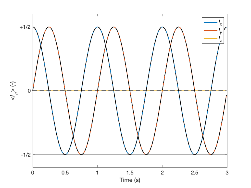
Lastly, we want to look at an important case: the evolution of systems with time-dependent Hamiltonians. In particular, we are interested in the situation where the Hamiltonian is not piece-wise time constant, but rather constantly evolving in time. As an example, we will simulate the evolution of a spin whose Larmor frequency evolves linearly in time from $\omega_{0,\textrm{i}}$ at time 0 to $\omega_{0,\textrm{f}}$ at time $t_\max$ ,

(19) $\begin{equation*}\omega_0(t) = \omega_{0,\textrm{i}} + (\omega_{0,\textrm{f}}-\omega_{0,\textrm{i}})\frac{t}{t_{\max}}.\end{equation*}$

This example is chosen because it is easy to treat, but it might not be particularly relevant in practice!

There are only a few differences in the script compared to the time-independent case. First, we need to define $\omega_{0,\textrm{i}}$ and $\omega_{0,\textrm{f}}$ in the beginning of the script. We will also define the time increments slightly differently for convenience. Instead of defining $dt$ and $K$ , we define $K$ and $t_\max$ and calculate $dt=t_{\max}K$ . More importantly, we cannot compute the Hamiltonian and the propagator in the beginning of the script, as it will change for each iteration $k$ . This must therefore be done within the for loop (see the next code snippet).

MATLAB
Python

omega0_i= 2*pi*0;   % Larmor freq at the beginning (rad.s-1)
omega0_f= 2*pi*6;   % Larmor freq in the end (rad.s-1)
tmax    = 3;        % Maximum time (s)
K       = 300;      % Number of increments (-)
S       = 1/2;      % Spin system - single spin 1/2

% Time axis and empty vectors to store results 
% of numerical propatation
dt      = tmax/K;
t       = dt*(0:K-1);
It      = zeros(3,K);

% Initial state
rho0    = I(S,'x');

% Observables
O{1}    = I(S,'x');
O{2}    = I(S,'y');
O{3}    = I(S,'z');

omega0_i= 2*pi*0;   % Larmor freq at the beginning (rad.s-1)
omega0_f= 2*pi*6;   % Larmor freq in the end (rad.s-1)
tmax    = 3;        % Maximum time (s)
K       = 300;      % Number of increments (-)
S       = 1/2;      % Spin system - single spin 1/2

% Time axis and empty vectors to store results 
% of numerical propatation
dt      = tmax/K;
t       = dt*(0:K-1);
It      = zeros(3,K);

% Initial state
rho0    = I(S,'x');

% Observables
O{1}    = I(S,'x');
O{2}    = I(S,'y');
O{3}    = I(S,'z');

omega0_i= 2*np.pi*0 # Larmor freq at the beginning (rad.s-1)
omega0_f= 2*np.pi*6 # Larmor freq in the end (rad.s-1)
tmax    = 3         # Maximum time (s)
K       = 300       # Number of increments (-)
S       = [1/2]     # Spin system - single spin 1/2

# Time axis and empty vectors to store results of numerical propagation
dt      = tmax/K;
t       = dt * np.arange(K)
It      = np.zeros((3, K))

# Initial state
rho0    = I(S,'x')

# Hamiltonian and propagator during dt
H0      = omega0*I(S,'z')
U0      = expm(-1j*H0*dt)

# Observables
O       = [I(S,'x'), I(S,'y'), I(S,'z')]

omega0_i= 2*np.pi*0 # Larmor freq at the beginning (rad.s-1)
omega0_f= 2*np.pi*6 # Larmor freq in the end (rad.s-1)
tmax    = 3         # Maximum time (s)
K       = 300       # Number of increments (-)
S       = [1/2]     # Spin system - single spin 1/2

# Time axis and empty vectors to store results of numerical propagation
dt      = tmax/K;
t       = dt * np.arange(K)
It      = np.zeros((3, K))

# Initial state
rho0    = I(S,'x')

# Hamiltonian and propagator during dt
H0      = omega0*I(S,'z')
U0      = expm(-1j*H0*dt)

# Observables
O       = [I(S,'x'), I(S,'y'), I(S,'z')]

Here is the key difference compared to the time-independent case. In the propagation loop, we compute the expectation values, but we need to compute the propagator before we can move the density matrix in time by $dt$ . We first compute the Larmor frequency at time $t_k$ using Eq. 19. Then, we calculate the Hamiltonian for this Larmor frequency and the corresponding propagator using Eq. 18. It’s not something that we usually like to do as computing the propagator can be very time consuming. For large spin systems, it can sometimes even take more than the propagation loop itself (it requires diagonalizing the Hamiltonian, which is computationally expensive for large matrices). So we only calculate the propagator at each step if we really need to.

MATLAB
Python

% Initialization of the system state
rho = rho0;

% Loop for propagation
for k = 1:K
    % Expectation values at time (k-1)*dt
    for i = 1:length(O)
        It(i,k) = real(trace(O{i}*rho));
    end

    % Hamiltonian and propagator during dt
    omega0  = omega0_i + (omega0_f-omega0_i)*t(k)/max(t);
    H0      = omega0*I(S,'z');
    U0      = expm(-1i*H0*dt);

    % Propagation during dt
    rho = U0*rho*U0';
end

% Initialization of the system state
rho = rho0;

% Loop for propagation
for k = 1:K
    % Expectation values at time (k-1)*dt
    for i = 1:length(O)
        It(i,k) = real(trace(O{i}*rho));
    end

    % Hamiltonian and propagator during dt
    omega0  = omega0_i + (omega0_f-omega0_i)*t(k)/max(t);
    H0      = omega0*I(S,'z');
    U0      = expm(-1i*H0*dt);

    % Propagation during dt
    rho = U0*rho*U0';
end

# Initialization of the system state
rho     = rho0

# Loop for propagation
for k in range(K):
    for i in range(3):
        # Expectation values at time (k-1)*dt
        It[i,k] = np.real(np.trace(O[i]@rho))
    
    # Hamiltonian and propagator during dt
    omega0  = omega0_i + (omega0_f - omega0_i) * t[k]/np.max(t);
    H0      = omega0 * I(S,'z');
    U0      = expm(-1j*H0*dt);
    
    # Propagate during dt
    rho = U0@rho@U0.T.conj()

# Initialization of the system state
rho     = rho0

# Loop for propagation
for k in range(K):
    for i in range(3):
        # Expectation values at time (k-1)*dt
        It[i,k] = np.real(np.trace(O[i]@rho))
    
    # Hamiltonian and propagator during dt
    omega0  = omega0_i + (omega0_f - omega0_i) * t[k]/np.max(t);
    H0      = omega0 * I(S,'z');
    U0      = expm(-1j*H0*dt);
    
    # Propagate during dt
    rho = U0@rho@U0.T.conj()

Finally, we plot the results. In this case, we don’t compare it with an analytical solution. For this simple single-spin case, an analytical solution can be found. This would require integrating the trajectory of the spins over time using the LvN equation (at least that’s how I would go about it). This is a much harder task than what we did to obtain the result of Eq. 7, which shows the usefulness of numerical simulations.

The resulting plot is shown below. It features an oscillation whose frequency increases with time, as expected from Eq. 19.

MATLAB
Python

% Plot of the results
figure(1), lw = 1.5;
plot(t,It,'LineWidth',lw)
yline([+1 -1]/2), ylim([-1 1]*0.6)
legend(['I_x', 'I_y', 'I_z'])
xlabel('Time (s)'), ylabel('<{\itI_\mu}> (-)')
yticks((-1:+1)/2), yticklabels({'-1/2','0','+1/2'})
set(gca,'FontSize',12)

% Plot of the results
figure(1), lw = 1.5;
plot(t,It,'LineWidth',lw)
yline([+1 -1]/2), ylim([-1 1]*0.6)
legend(['I_x', 'I_y', 'I_z'])
xlabel('Time (s)'), ylabel('<{\itI_\mu}> (-)')
yticks((-1:+1)/2), yticklabels({'-1/2','0','+1/2'})
set(gca,'FontSize',12)

# Plot of the results
plt.figure(1)
lw = 1.5
plt.plot(t, It.T, linewidth=lw)
plt.axhline(y=1/2, color='gray', linestyle='--')
plt.axhline(y=-1/2, color='gray', linestyle='--')
plt.legend(['I_x', 'I_y', 'I_z'])
plt.xlabel('Time (s)')
plt.ylabel('<I_μ> (-)')
plt.yticks(np.arange(-1, 2, 1) / 2, ['-1/2', '0', '+1/2'])
plt.gca().tick_params(labelsize=12)
plt.show()

# Plot of the results
plt.figure(1)
lw = 1.5
plt.plot(t, It.T, linewidth=lw)
plt.axhline(y=1/2, color='gray', linestyle='--')
plt.axhline(y=-1/2, color='gray', linestyle='--')
plt.legend(['I_x', 'I_y', 'I_z'])
plt.xlabel('Time (s)')
plt.ylabel('<I_μ> (-)')
plt.yticks(np.arange(-1, 2, 1) / 2, ['-1/2', '0', '+1/2'])
plt.gca().tick_params(labelsize=12)
plt.show()

How to choose dt

Conclusion

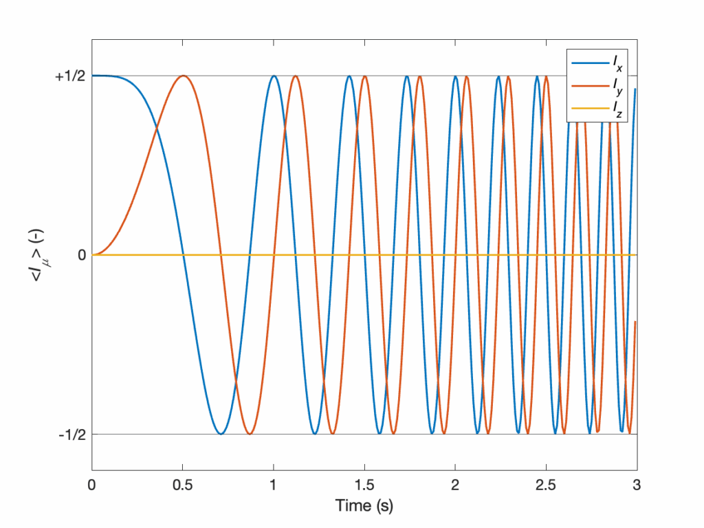
In this post, we have seen how the density matrix evolves in time with different methods, either using cyclic commutation relations or using the solution to the Liouville-Von Neuman equation. In the next posts, we’ll explore how the density matrix can be computed for coupled spins and for large spin ensembles. Stay tuned!

Time evolution of the density matrix

Liouville-Von Neumann equation

Calculation details

LvN equation and cyclic commutation

Proof

Calculation details

Solution to the LvN equation

Calculation details

Numerical simulation of time-independent Hamiltonian

Numerical simulation of time-dependent Hamiltonian

How to choose dt

Conclusion

Leave a Reply Cancel reply

Artist Credit:

Contact:

Website designed and developed by:

Time evolution of the density matrix

Liouville-Von Neumann equation

Calculation details

LvN equation and cyclic commutation

Proof

Calculation details

Solution to the LvN equation

Calculation details

Numerical simulation of time-independent Hamiltonian

Numerical simulation of time-dependent Hamiltonian

How to choose dt

Conclusion

Leave a Reply Cancel reply

Artist Credit:

Contact:

Website designed and developed by:

Quantum Insights