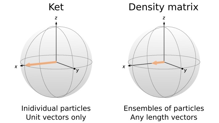
Hello! Welcome back to our post series introducing the density matrix. In the previous post, the density matrix was introduced, and we saw how it serves as a tool for considering ensembles of spins where the ket formalism may break down. We then constructed the density matrix for some standard spin states. However, it may still be unclear how to extract observables from the density matrix, or how the density matrix evolves in time – both key concepts to actually using the density matrix to understand magnetic resonance experiments. In this post, we will see how the density matrix can be used to calculate expectation values (and thus extract observables), while the next post will explore time evolution in the density matrix formalism.
Previously, we showed how to calculate the density matrix for a state ![]() by expressing
by expressing ![]() as a column vector and
as a column vector and ![]() as a row vector and taking the Kronecker product to express
as a row vector and taking the Kronecker product to express ![]() as a matrix. We can also calculate the matrix elements of
as a matrix. We can also calculate the matrix elements of ![]() by remembering that
by remembering that ![]() is an operator. As we recall, the matrix elements of an operator
is an operator. As we recall, the matrix elements of an operator ![]() can be expressed as
can be expressed as
(1) ![]()
where ![]() and
and ![]() represent the eigenstates of the basis we are using to express the operator. We can extend this definition to the density matrix, and get
represent the eigenstates of the basis we are using to express the operator. We can extend this definition to the density matrix, and get
(2) ![]()
From this form, we see that the matrix elements of the density matrix for a state ![]() are related to the projection of the different eigenstates of our basis onto the state
are related to the projection of the different eigenstates of our basis onto the state ![]() .
.
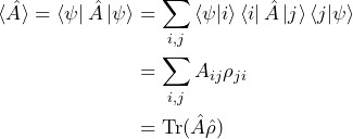
With the form of the density matrix introduced in Eq. 2, we can now calculate the expectation value of an observable associated with operator ![]() using our density matrix formalism. First, we recall two things. One, the expectation value of an operator
using our density matrix formalism. First, we recall two things. One, the expectation value of an operator ![]() for a state
for a state ![]() is
is
(3) ![]()
and two, we can express the identity as the summation over the outer product of each of our basis states
(4) ![]()
We will then use that we can insert a copy (or two) of the identity into our equations without impacting the equalities (i.e. multiplying by ![]() has no effect!).
has no effect!).
(5) 
In the above, we have used that inner products are complex numbers and there multiplication is commutative. We also have introduced the trace of a matrix, which is the sum of its diagonal elements. In our case, we are tracing over the matrix product of our observable operator ![]() and our density matrix
and our density matrix ![]() . Since the trace is an easy value to calculate (simply a sum along the diagonal), Eq. 5 provides a straightforward epxression for using the density matrix to find expectation values.
. Since the trace is an easy value to calculate (simply a sum along the diagonal), Eq. 5 provides a straightforward epxression for using the density matrix to find expectation values.
There are multiple ways to show that ![]() is a valid equation. One approach is that we can calculate the outer product for each state expressed in vector notation. The
is a valid equation. One approach is that we can calculate the outer product for each state expressed in vector notation. The ![]() basis state,
basis state, ![]() , can be expressed in vector notation as
, can be expressed in vector notation as
(6) 
where we have a ![]() on the
on the ![]() element and a
element and a ![]() everywhere else. Then, it is clear that the outer product
everywhere else. Then, it is clear that the outer product ![]() will be a matrix of all
will be a matrix of all ![]() ‘s, except for the
‘s, except for the ![]() element of the diagonal, which will be a
element of the diagonal, which will be a ![]() . Summing over all the
. Summing over all the ![]() basis states then gives the matrix with
basis states then gives the matrix with ![]() ‘s on the diagonal, and
‘s on the diagonal, and ![]() ‘s for every other element. This matrix is the
‘s for every other element. This matrix is the ![]() -dimensional identity matrix, so we must have
-dimensional identity matrix, so we must have
(7) ![]()
We will now use the expression in Eq. 5 to calculate the expectation value of some example states and operators. We will consider the expectation values of the operator ![]() for the states
for the states ![]() and
and ![]() . First, we need to find the density matrix for each of these states, working in the
. First, we need to find the density matrix for each of these states, working in the ![]() basis as usual. For
basis as usual. For ![]() , we saw in the previous post that we have
, we saw in the previous post that we have
(8) ![]()
while for ![]() we have
we have
(9) ![]()
As we have previously seen, we can express the operator ![]() in matrix form as
in matrix form as
![]()
where we are using the convention ![]() . Now, using Eq. 5, we can calculate the expectation value of
. Now, using Eq. 5, we can calculate the expectation value of ![]() for each state. For state
for each state. For state ![]() , we get
, we get
(10) ![]()
which is indeed the expectation value of state ![]() for the
for the ![]() operator. For
operator. For ![]() , we get
, we get
(11) ![]()
which again is the proper expectation value, this time for the state ![]() (recall that we are using
(recall that we are using ![]() and that the expectation value for this eigenstate is actually
and that the expectation value for this eigenstate is actually ![]() ).
).
The same calculations are shown in the code snippet below using MATLAB and Python/Numpy.
% Definition of kets
ket_1     = [1 ;0];
ket_2     = [1 ; -1]/sqrt(2);

% Corresponding density matrices
rho_1     = ket_1*ket_1';
rho_2     = ket_2*ket_2';

% Angular momentum operator
I_x       = [0 1; 1 0]/2;

% Expectation values
O_1       = trace(I_x*rho_1);
O_2 = trace(I_x*rho_2);# Required package for numerical calculations
import numpy as np
# Definition of kets
ket_1 = np.array([1, 0])
ket_2 = np.array([1, -1])/np.sqrt(2)
# Corresponding density matrices
rho_1 = np.outer(ket_1, ket_1)
rho_2 = np.outer(ket_2, ket_2)
# Angular momentum operator
I_x = np.array([[0, +1/2],[ +1/2, 0]])
# Expectation values
O_1 = np.trace(I_x@rho_1)
O_2 = np.trace(I_x@rho_2)In this post, we have seen how to use the density matrix to calculate the expectation value of an operator by taking the trace of the product of the density matrix and the operator in question, and went through some simple example calculations. Now, the density matrix is a bit more useful, as we can use it to extract measurable values! In the next post, we will explore time evolution with the density matrix. Combined with what we learned here, we will then be able to use the density matrix formalism to simulate magnetic resonance experiments.