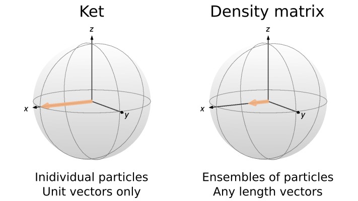
In our first post series, we presented the postulates of quantum mechanics. In doing so, we introduced the ket formalism, and showed how we can use it to describe and understand some experiments involving spins. However, this formalism is only applicable to individual system of particles; it can’t be used to describe a large ensemble of particles. In this post, we will show why this is the case. We will then introduce the density matrix formalism, which allows us to describe experiments involving ensembles in a convenient way. This post is the first of a series on the density matrix formalism. Dealing with ensembles is important as most magnetic resonance experiments are performed on large ensemble of (nearly) identical spin systems.
Think of a sample consisting of a large number of non-interacting spins 1/2, all polarized in the same direction. The ket corresponding to the state of each of these spins  can be written as
(1) 
where  is the global phase of spin . Can we construct a ket that would correspond to the average over all kets in the sample? That’s what we are explicitly doing below, assuming the number of particles tends to infinity, which allows us to jump from a sum to an integral,
(2) 
What happened here? The average over all kets in the sample is a 0 ket, because the average of the global phase – which is random – is 0. This can be seen as the particle “disappearing” due to the averaging. That’s certainly not a useful approach. As we will see, to describe this sort of ensemble, we can express the state of the system using the density matrix formalism. Contrary to the ket approach, the density matrix – spoiler alert – will survive the averaging procedure. Note that if the global phase was the same for the particles, the ket formalism would collapse when averaging over the ensemble.
Let  represent the state of all the copies of the quantum mechanical system we are studying. These copies may be identical or have some differences that we don’t specify for now, like the global phase. They can also vary in more fundamental ways (as we will see in future posts). In any case, the corresponding density matrix is defined as
(3) 
where is the index of the kth particle in the sample and  is the total number of particles in the sample.
  is the product of a row and a column vector, a square matrix with dimension
  . As in Eq. 2, the bar represents the average over all copies of the system.
Now, let’s look at how the phase factor  affects the ket-bra product. If two kets
  and
and  are identical up to the phase factor, then we have
  , where
  is the global phase difference between the two kets. The density matrix of particle is then
(4) 
which is equal to the density matrix of particle  . This shows that the density matrix is independent of the global phase of the ket. Coming back to example that we took above of a large ensemble of isolated spins 1/2 all pointing in the same direction. We already know that we don’t need to calculate what happens to the phase factor, the ket-bra product will make it disappear before we take the average over all spins. We get
(5) 
The density matrix does not collapse to 0, which looks promising for the description of ensembles.
Let’s look at some simple examples of density matrices for some familiar states. In a previous post, we defined states corresponding to a spin pointing along the three different Cartesian axes
(6) 
To calculate the density matrix corresponding to these states, we don’t need to worry about the global phase as we know it disappears when we calculate the ket-bra. For the same reason, we don’t need to write the bar either. We get
(7) 
Something very important appears here. When calculating the density matrix corresponding to the ket of certain spin states, we obtain expressions that contain angular momentum operators. In other words, the angular momentum operators not only represent elements in the Hamiltonians acting on spins, but they can also be used to represent spin state in the density matrix formalism. This can be the source of some confusion and certainly was confusing to me when I first learnt about all this! Note that we often use the terms density operator and density matrix interchangeably in the matrix representation of quantum mechanics.
The code snippet below shows how to write these operations in MATLAB and Python (using Numpy). Note that in MATLAB, row and column vectors are distinct, so the bra can be computed as the complex conjugate of the ket before taking their product (in the appropriate order). In Numpy/Python, there is no difference between row and column vectors, so the product between the bra and the ket must be computed using the outer product function. Otherwise, the product between the bra and the ket returns their scalar (inner) product, i.e., a number, while we need a  matrix.
% Definition of kets
ket_alpha = [1; 0];
ket_beta  = [0; 1];
ket_x     = (ket_alpha + ket_beta)/sqrt(2);
ket_y     = (ket_alpha + 1i*ket_beta)/sqrt(2);
ket_z     = ket_alpha;

% Corresponding density matrices
rho_x     = ket_x*ket_x';
rho_y     = ket_y*ket_y';
rho_z = ket_z*ket_z';# Required package for numerical calculations
import numpy as np
# Definition of kets
ket_alpha = np.array([1, 0])
ket_beta = np.array([0, 1])
ket_x = (ket_alpha+ket_beta)/np.sqrt(2)
ket_y = (ket_alpha+1j*ket_beta)/np.sqrt(2)
ket_z = ket_alpha
# Corresponding density matrices
rho_x = np.outer(ket_x, ket_x.conj())
rho_y = np.outer(ket_y, ket_y.conj())
rho_z = np.outer(ket_z, ket_z.conj())We have defined the density operator. That’s the tip of the iceberg. In the next posts, we will show how expectation values are extracted from the density matrix and we will derive an equivalent to the Schrödinger equation for the density matrix (the so-called Liouville-Von Neumann equation). This will allow us to perform with the density matrix all the operations that we defined for the ket in the post series on the postulates of quantum mechanics, and perform spin dynamics simulation. We will see that the state of the system is often more intuitively captured using the density matrix. Then, we will go further and see how the density matrix allows us to describe large ensembles, even when they are disordered. Again, we will see that in this case the ket formalism completely breaks down.


