April 7th, 2025

The Bloch sphere

Author: Josh Straub
Editor: Quentin Stern

Hello! In this post I will be discussing one of the foundational tools for visualizing two-level quantum systems such as a spin 1/2 particle, the Bloch sphere. The Bloch sphere is powerful in that it provides an easy-to-understand visual picture of the full state space of a single qubit. As such, the Bloch sphere is ubiquitous in both magnetic resonance and quantum information science as a visual aid whenever discussing two-level systems.

This post will begin by introducing how we can represent an arbitrary pure state with the Bloch sphere. From there, we will consider some example states, and learn how to move between Dirac (i.e. bra-ket) notation and the Bloch sphere representation. Next, we will show how mixed states are represented by the Bloch sphere, and how we can use the Bloch sphere as a handy tool for thinking about how mixed or pure a state is. Finally, we will wrap up with a brief discussion of spins with spin number $>1/2$ . Hopefully this post will serve as a good introduction for those new to the Bloch sphere or as a helpful reminder for those already familiar.

Defining a state with the Bloch sphere

Let’s start by considering some arbitrary, normalized state $\ket{\psi} = c_\alpha \ket{0} + c_\beta \ket{1}$ , where $|c_\alpha|^2 + |c_\beta|^2=1$ . Now, up to a global phase of our state, we can take $c_\alpha$ to be real and positive, so that we have $0 \leq c_\alpha \leq 1$ . This means that we can define some angle $0 \leq \theta \leq \pi$ so that $c_\alpha = \cos(\theta/2)$ . By the normalization requirement, this means that $c_\beta = e^{i \phi} \sin(\theta/2)$ , where we have introduce a second angle $0 \leq \phi < 2\pi$ which allows us to define an arbitrary phase between $\ket{0}$ and $\ket{1}$ . Thus, we see with two angles, $\theta$ and $\phi$ , we are able to describe any arbitrary, normalized state $\ket{\psi}$ of a two level system. Looking at the bounds on $\theta$ and $\phi$ , you might recognize that the full phase space of these two angles defines the surface of a sphere!

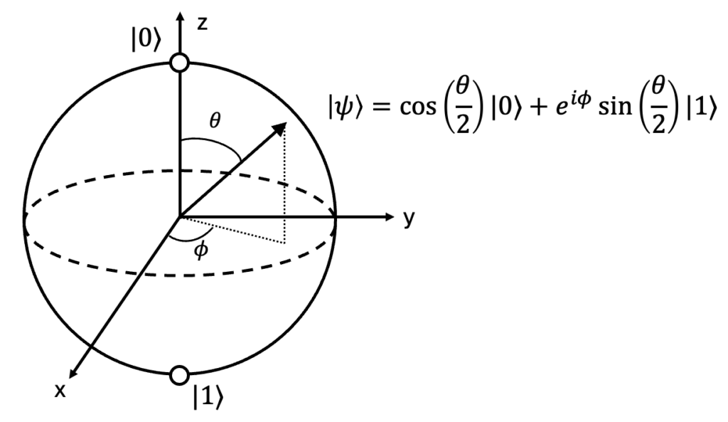
This sphere is exactly the Bloch sphere, shown below. As you can see, the top of the sphere defines the state $\ket{0}$ , while the bottom of the sphere is the state $\ket{1}$ . As always, we can think of $\ket{0}$ and $\ket{1}$ as spin down and spin up, respectively. As we just showed above, the surface of the Bloch sphere can represent any state $\ket{\psi}$ of a two-level system. (Technically any pure state. We will discuss mixed states below). The state is often represented as a vector from the origin to the point on the surface of the Bloch sphere that defines the state. The angle between the $\ket{0}$ state (i.e. $z$ -axis) and the vector is $\theta$ , while the angle in the $xy$ -plane is $\phi$ , where $\phi = 0$ is defined by the $x$ -axis. We’ve turned the mathematically defined state, $\ket{\psi} = c_\alpha \ket{0} + c_\beta \ket{1}$ , where we have to process the complex numbers $c_\alpha$ and $c_\beta$ to understand the state, into a state defined as a point on a familiar easy to visualize object, a sphere.

A couple of important notes before we look at some different state representations with the Bloch sphere. First, we saidabove that we can represent any pure state with the Bloch sphere, meaning that we can represent the full Hilbert space of a spin 1/2 particle. However, recall that this is a representation up to a global phase, since we defined $c_\alpha$ as real. Thus, we are really able to represent the full projective Hilbert space of a spin 1/2 particle. A subtle, but sometimes important, difference.

Second, I wanted to mention the Riemann sphere, the mathematical “parent” object of the Bloch sphere. The Riemann sphere is a way to visualize the complex plane as a projection onto a sphere, with the bottom of the sphere at $0$ , top of the sphere at $\infty$ , and the $x-y$ plane representing the sign and magnitude of the real/imaginary parts of the complex number. In the case of the Bloch sphere, we’ve mapped the Riemann sphere onto our two-level quantum system, but the Riemann sphere also finds other applications in complex analysis and physics.

Now, let’s return to our spin 1/2 particle and consider a couple of the eigenstates of our angular momentum operators and translate them into representations on the Bloch sphere. Clearly, the eigenstates of $\hat{I}_z$ , our spin down and spin up states, are $\ket{0}$ and $\ket{1}$ . But what about $\hat{I}_x$ and $\hat{I}_y$ ? Let’s take the state $\ket{-x} = \frac{1}{\sqrt{2}}(\ket{0} - \ket{1})$ that was introduced in the post series on the postulates of quantum mechanics. Since this is an equal superposition of $\ket{0}$ and $\ket{1}$ , we must have that $\theta = \pi/2$ . Then, we note that the phase between $\ket{0}$ and $\ket{1}$ is $-1 = e^{i\pi}$ , so that $\phi = \pi$ . Returning to our Bloch sphere, we see that this state is represented by a vector pointing along the negative $x$ -axis – which makes perfect sense for the state $\ket{-x}$ .

Similarly, we can consider the eigenstate of $\hat{I}_y$ , $\ket{+y} = \frac{1}{\sqrt{2}}(\ket{0}+i \ket{1})$ . Again, we see that there is an equal superposition of $\ket{0}$ and $\ket{1}$ , indicating that $\theta = \pi/2$ . The phase between $\ket{0}$ and $\ket{1}$ is $i = e^{i\pi/2}$ , so that $\phi = \pi/2$ . Referring back to the Bloch sphere, we recognize that this state is represented by a vector pointing along the positive $y$ -axis.

These are relatively simple examples, and you probably could’ve guessed the Bloch sphere representation. But it is nice to confirm that the Bloch sphere naturally corresponds with the angular momentum eigenstates. For more complex states, it might not be so easy to know $\theta$ and $\phi$ by inspection. But there is a relatively simple formula for calculating them, which you can deduce from an inspection of the Bloch sphere and some trigonometry. For an arbitrary state $\ket{\psi} = c_\alpha \ket{0} + c_\beta \ket{1}$ , our state is defined on the Bloch sphere by the angles

(1) $\begin{equation*} \begin{split}& \theta/2 = \arctan(\frac{|c_\beta|}{|c_\alpha|}) \\& \phi = \phi_\beta - \phi_\alpha\end{split} \end{equation*}$

where we have used that complex numbers $c_\alpha$ and $c_\beta$ can be expressed as $c_\alpha = |c_\alpha| e^{i\phi_\alpha}$ and $c_\beta = |c_\beta| e^{i\phi_\beta}$ .

Since the Bloch sphere can represent any pure state $\ket{\psi}$ , it can also represent the evolution of a pure state. For instance, if we are initially in the state $\ket{0}$ (spin down), we can imagine the action of a $(\pi/2)_y$ pulse nutating our state to be aligned with the $x$ -axis. As such, the Bloch sphere is a powerful tool for visualizing not just static states but their evolution as well. Look out for a future post will explore simulating and visualizing evolution using the Bloch sphere!

Mixed states

Thus far, we have restricted our discussion to pure states, and have used the terminology of the the Bloch sphere. However, this representation scheme can also be used for mixed states. But now we must consider the Bloch ball, which includes not only the spherical surface but the interior of the sphere as well. Recall that pure states are states that can be represented by a ket, such as $\ket{\psi}$ above, while mixed states are statistical ensembles of pure states. For instance, we could have a mixed state where we have half our particles in the state $\ket{0}$ and the other half in $\ket{1}$ . If we pick one at random, there is a $50\%$ chance that we will observe the state $\ket{0}$ . At first, this may seem like the same thing as the superposition state $\ket{\psi} = \frac{1}{\sqrt{2}}(\ket{0}+\ket{1})$ . But the superposition state will evolve differently, and will be represented differently when we consider the density matrix. Even though both cases have a $50\%$ chance of observing a particle in the state $\ket{0}$ , their physical behavior is quite distinct.

So, how do we use the Bloch ball to represent mixed states? In the case of mixed states, let us consider the density operator, as a single ket is no longer an appropriate descriptor. An arbitrary mixed state $m$ for a two-level system can be defined by the density operator $\hat{\rho}_m = \frac{1}{2} (\hat{\mathbb{I}} + \vec{a} \cdot \hat{\vec{\sigma}})$ , where $\mathbb{I}$ is the identity matrix, $\vec{\sigma}$ are the three Pauli matrices, and $\vec{a}=(a_x,a_y,a_z)$ is a vector with magnitude $|\vec{a}|^2 \leq 1$ that defines the state. Expanding this representation, we find

(2) $\begin{equation*}\hat{\rho}_m = \frac{1}{2} \begin{pmatrix} 1+a_z & a_x - i a_y \\ a_x + i a_y & 1-a_z \end{pmatrix}\end{equation*}$

The magnitude of $\vec{a}$ will define the length of the state vector in the Bloch ball. In the limit of $|\vec{a}|=1$ , the state vector will be at the surface of the sphere, and we recover a pure state. In the limit of the mixed state described above that has half the particles in the state $\ket{0}$ and the other half in $\ket{1}$ , a total statistical mixture with no superposition, the density matrix is $\hat{\rho}_m = \frac{1}{2} \begin{pmatrix} 1 & 0 \\ 0 & 1 \end{pmatrix}$ . We recognize that this means that $\vec{a} = 0$ . In this case, our state is represented by the point at the origin of the Bloch ball (really a vector with zero length starting at the origin).

Now, there are many mixed states that aren’t just an equal statistical mixture of $\ket{0}$ and $\ket{1}$ , where some states are more probable than others, or where the pure states that make up the ensemble also have some degree of superposition. These states will have $0<|\vec{a}|<1$ and be represented somewhere between the origin and the surface of the Bloch sphere. The closer to the surface ( $|\vec{a}|$ closer to $1$ ) the “purer” the mixed state, while the closer to the origin ( $|\vec{a}|$ closer to $0$ ), the more “mixed” the state is. In this sense, the Bloch ball is a very useful tool to think about just how pure or mixed a state is.

One more note on the definition of the Bloch sphere given in equation (2). From this definition, we can see that the Bloch sphere is essentially a 3-dimensional map of the angular momentum operators (the Pauli matrices and spin 1/2 angular momentum operators differ by just a factor of $\hbar/2$ ). Thus, we can almost think of the Bloch sphere in a classical physics sense, with $\vec{a}$ defining the classical projection of our three angular momentum operators. However, this classical picture is not always appropriate – say, in the description of a measurement of angular momentum of a single particle – so be cautious!

What about spins > 1/2?

Throughout this discussion, we have only talked about two-level systems, but plenty of interesting spin physics occurs in spin systems with $S>1/2$ . So can the Bloch sphere help us think about them? Unfortunately, the answer is no (unless you feel like you can visualize objects in 4 dimensions). Let’s consider the case of a pure state of a spin 1 particle. In this case, we can write an arbitrary state as $\ket{\psi} = c_\alpha \ket{-1} + c_\beta \ket{0} + c_\gamma \ket{1}$ , where the states $\ket{i}$ are the Zeeman eigenstates and the coefficients are complex numbers. To represent this state using real numbers, we need four parameters – the magnitudes of $c_\alpha$ and $c_\beta$ (the magnitude of $c_\gamma$ is then set by the normalization condition) and the relative phase between $\ket{-1}$ and $\ket{0}$ and $\ket{-1}$ and $\ket{1}$ . Thus, even if we restrict ourselves to pure states, we would need to be able to visualize a 4-dimensional object for an equivalent visual representation of a spin 1 particle. And for higher spin number, the required dimension just gets larger. For most of us, that’s more complicated than the mathematical representation, and so there is no real practical extension of the Bloch sphere to $S > 1/2$ .

Conclusion

With that, we will wrap up our introduction to the Bloch sphere. Here, we saw that the Bloch sphere (or Bloch ball) is a powerful tool for the visualization of two-level systems, such as a spin 1/2 particle, for both pure and mixed states. This natural visual representation of two-level systems makes the Bloch sphere a ubiquitous tool across magnetic resonance and quantum information science to understand states and their evolution. Stay tuned for future posts that go into depth on the simulation and visualization of state evolution with the Bloch sphere!

The Bloch sphere

Defining a state with the Bloch sphere

Mixed states

What about spins > 1/2?

Conclusion

Leave a Reply Cancel reply

Artist Credit:

Contact:

Website designed and developed by:

The Bloch sphere

Defining a state with the Bloch sphere

Mixed states

What about spins > 1/2?

Conclusion

Leave a Reply Cancel reply

Artist Credit:

Contact:

Website designed and developed by:

Quantum Insights