April 4th, 2025

Simulating a simple 1D NMR spectrum

Author: Quentin Stern
Editor:

Welcome to this first post on real NMR simulation! In this post, we will see how to simulate from scratch the NMR spectrum of a single spin in a magnetic field $B_0$ , using the density matrix formalism. We will detail each step and break down the script into code snippets, both in MATLAB and Python. These scripts makes use of a function that is not detailed in this post, to compute angular momentum operators. This function, called I, was presented in a previous post in detail. The full Python script is available here (it can be run and modified directly in your browser, provided you have a Google account) and the full MATLAB script is available here.

Experimental vs simulated process

Modern NMR experiments use radio frequency pulses to perturb the system, before measuring the oscillations of the perturbed system. In the simplest case, the system is initially at thermal equilibrium, with the magnetization aligned with the magnetic field (along the $z$ axis by convention). A short radio frequency pulse tilts the magnetization to plan perpendicular to the magnetic field. Following this, the magnetization freely precesses about the magnetic field, at the Larmor frequency of the nuclear spins (typically, hundreds of MHz). Doing so, it generates an oscillating voltage in the pick-up coil of the NMR probe, the same coil that was use to apply the pulse. This signal is demodulated down to audio frequencies (< MHz) and recorded by a digitizer. Finally, the resulting free induction decay (FID) is Fourier transformed to obtain the NMR spectrum.

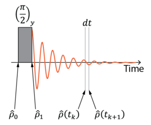
The most common way – although not unique -, to simulate this type of experiments is by time propagation in Liouville space. We start by computing the density matrix corresponding to the spin system at equilibrium, with the magnetization aligned along the $z$ axis. We apply a pulse to the density matrix just as we do in the experiment to bring the spins to the transverse plan, using the pulse propagation operator. Then, we apply the free evolution propagation operator in small time steps corresponding to the digitization steps in the experiment. At each time point, the expectation value corresponding to what the pick coil measures are extracted from the density matrix. This collection of points forms the simulated FID. The exact same processing that is applied to the experimental FID is applied to the simulated FID to obtain a spectrum.

Definition of the variables

The first block of the script defines the variables that are used throughout the script. We describe them briefly here, but they will surely become clearer when they are used in the next sections.

The first one, SS, is a list containing the spin number of the spins in the system. In this case, we have a single spin 1/2. This is required by the function I that computes the angular momentum operator. P0 is the polarization of the spins, it is used to compute the initial density matrix. It’s typically a small number (on the order of ppm to hundreds of ppm). Its only influence on the spectrum is to scale it up and down. Omega0 is the offset frequency of the spins relative to the carrier $\omega_\textrm{ref}$ ,

(1) $\begin{equation*}\Omega_0 = \omega_0 - \omega_\textrm{ref},\end{equation*}$

where $\omega_0$ is the nuclear Larmor frequency. Under free precession, the spins rotate at the offset frequency rather than at the Larmor frequency, because the simulation is performed in the rotating frame. Here, the offset frequency is set to $\Omega_0/(2/\pi) = 10~\textrm{Hz}$ . The sampling frequency f determines how many points are acquired per second. Just as in an experiment, it is equal to the width of the spectrum. It needs to be twice the largest frequency we expect in the spectrum to avoid refolding or aliasing (as per the Nyquist criterion). lb is the line broadening applied to the spectrum. Because the simulation that we are setting up does not include relaxation effects, we use line broadening or apodization to make the signal decay to 0, and look like an FID (which decays to 0). K and L are the number of points in the FID and the spectrum, respectively. When K is larger than L, the FID is “zero-filled”, that is, we have added zeros in the end of the FID to make the spectrum smoother. The total length of the FID is

(2) $\begin{equation*}t_\textrm{max} = \frac{K-1}{f}.\end{equation*}$

MATLAB
Python

% Definition of variables
SS      = 1/2;      % Spin system
P0      = 1e-6;     % Initial polarization, -
Omega0  = 2*pi*10;  % Offset frequency, rad.s-1
f       = 100;      % Sampling frequency/spectral width, Hz
lb      = 1;        % Lorentzian line broadening, Hz  
K       = 2^9;      % Number of points in the FID, -
L       = K*4;      % Number of points in the spectrum, -

# Variable definition
SS      = [1/2]       # Spin system
P0      = 1e-6        # Initial polarization, -
Omega0  = 2*np.pi*10  # Offset frequency, rad.s-1
f       = 100         # Sampling frequency/spectral width, Hz
lb      = 1           # Lorentzian line broadening, Hz
K       = 512         # Number of points in the FID, -
L       = K*4         # Number of points in the spectrum, -

Initial state

The initial state of the system, for an ensemble of isolate nuclear spin, is

(3) $\begin{equation*}\hat{\rho}_0 = \frac{\hat{1}}{2}+P_0\hat{I}_z,\end{equation*}$

where $P_0$ is the nuclear Boltzmann polarization and $\hat{I}_z$ is the $z$ angular momentum operator. However, the identity operator $\hat{1}$ is often omitted as it gives rise to no observable signal and it does not evolve with time, yielding

(4) $\begin{equation*}\hat{\rho}_0 = P_0\hat{I}_z.\end{equation*}$

MATLAB
Python

% Initial state - density matrix
rho0 = P0*I(SS,1,'z');

# Initial state - density matrix
rho0 = P0*I(SS,0,'z')

Excitation pulse

We then apply a $\pi/2$ pulse to bring the magnetization into the transverse plan. This is done using the time evolution propagator of the pulse Hamiltonian. The pulse Hamiltonian reads

(5) $\begin{equation*}\hat{H}_1 = \omega_1\hat{I}_y,\end{equation*}$

where $\omega_1$ is the nutation frequency of the pulse. The corresponding propagator reads

(6) $\begin{equation*}\begin{split}\hat{U}_1 &= \exp{(-i\hat{H_1}t_\textrm{p})}\\&= \exp{(-i\omega_1\hat{I}_yt_\textrm{p})}\\&= \exp{(-i\beta\hat{I}_y)},\end{split}\end{equation*}$

where $t_p$ is the length of the pulse and $\beta = \omega_1 t_p$ is the nutation angle of the pulse, which we set to $\pi/2$ . The fact that the free evolution Hamiltonian is not included during the pulse means that the pulse rotates the spins instantaneously, like if time was stopped during the pulse. This concept is called hard pulses.

Note that the operation exp is a matrix exponential, which is different from an element-by-element exponentiation. As such, special care must be take when coding it as element-by-element exponentiation also exists in MATLAB and Numpy.

The state of the system after the pulse is given by the solution to the Liouville-Von Neumann equation

(7) $\begin{equation*}\hat{\rho}_1 = \hat{U}_1 \hat{\rho}_0\hat{U}_1^*.\end{equation*}$

MATLAB
Python

% Excitation pulse propagator
Up   = expm(-1i*pi/2*I(SS,1,'y')); 

% Excitation pulse propagation
rho1 = Up*rho0*Up';

# Excitation pulse propagator
Up   = expm(-1j*np.pi/2*I(SS,0,'y'))

# Excitation pulse propagation
rho1 = Up@rho0@Up.T.conj()

Free evolution propagator

The free evolution propagator will make the system move in time by one time increment $dt$ in the propagation loop (see below). To compute it, we first need to define the free evolution Hamiltonian, which only contain the Zeeman contribution. In the rotating frame, it reads

(8) $\begin{equation*}\hat{H}_0 = \Omega_0\hat{I}_z.\end{equation*}$

The length of the time increments is the inverse of the sampling frequency (which is itself equal to the spectral width defined above)

(9) $\begin{equation*}dt = \frac{1}{f}.\end{equation*}$

The free evolution propagation is then calculated as for the pulse propagator above

(10) $\begin{equation*}\hat{U}_0(dt) = \exp{(-i\hat{H}_0dt)}.\end{equation*}$

MATLAB
Python

% Free evolution Hamiltonian
H0 = Omega0*I(SS,1,'z');

% Free evolution time propagator during dt
dt = 1/f;
U0 = expm(-1i*H0*dt);

# Free evolution Hamiltonian
H0 = Omega0*I(SS,0,'z')

# Free evolution time propagator during dt
dt = 1/f
U0 = expm(-1j*H0*dt)

Observable

The pick coil of an NMR probe is usually sensitive to the sample magnetization along a single axis. In liquid-state probes, this axis is perpendicular to the $B_0$ field. Let’s define this axis as the $x$ axis. We should naturally define the observable operator as $\hat{I}_x$ . However, the electronics in the spectrometer artificially constructs the orthogonal component, as if our NMR probe had two pick-up coils, one sensitive to $x$ and the other sensitive to $y$ . The operator corresponding to the resulting complex signal is therefore

(11) $\begin{equation*}\hat{O} = \hat{I}_x+i\hat{I}_y=\hat{I}_+.\end{equation*}$

This has the great advantage that complex signals distinguish positive and negative frequencies. If only the real part was recorded, the NMR spectrum would be symmetric around the center, which could lead to signal overlapping.

MATLAB
Python

% Observable operator
O  = I(SS,1,'+');

# Observable operator
O  = I(SS,0,'+')

Free evolution

The core the simulation happens here. We first define an empty vector to store the FID, then we initialize the density matrix at the beginning of the free evolution time period $\hat{\rho}(0)$ as the density matrix immediately after the pulse $\hat{\rho}_1$ . Then, a for loop repeats the same operation K times. At each iteration, the expectation value is extracted from the density matrix using

(12) $\begin{equation*}\braket{\hat{I}_+(t_k)}=\textrm{Tr}\{\hat{I}_+\hat{\rho}(t_k)\}.\end{equation*}$

The system is moved in time by one time increment $dt$ using the same procedure as for the pulse propagation

(13) $\begin{equation*}\hat{\rho}(t_{k+1}) = \hat{U}_0(dt) \hat{\rho}(t_k)\hat{U}_0(dt)^*,\end{equation*}$

where the time points along the FID are defined as

(14) $\begin{equation*}t_k=(k-1)dt,\end{equation*}$

where $k\in[1:K]$ .

MATLAB
Python

% Propagation
% Empty vector to store FID
FID = zeros(1,K);

% Loop for free evolution
rhok= rho1;
for k=1:K
    % Extract expactation value
    FID(k) = trace(O*rhok);

    % Propagate during dt
    rhok = U0*rhok*U0';
end

# Propagation
# Empty vector to store FID
FID = np.zeros(K,dtype=complex)

# Loop for free evolution
rhok = rho1
for k in range(K):
    # Extract expactation value
    FID[k] = np.trace(O@rhok)

    # Propagate during dt
    rhok = U0@rhok@U0.T.conj()

Apodization

Apodizing the signal (which is also referred to as applying a window function) is necessary for two reasons. First, as stated in the intro, the signal does not decay to zero because our simulation does not account for relaxation. If we don’t correct this, the spectrum will feature non-Lorentzian signals, more specifically sinc patterns. This is corrected by applying line broadening to the FID. We first define an effective T₂ (in s) that will produce the desired line broadening $\delta_{1/2}$ in Hz

(15) $\begin{equation*}T_2=\frac{1}{\pi \delta_{1/2}}.\end{equation*}$

We then compute the time axis $t$ corresponding to the points in the FID, using Eq. 14. Finally, we multiply the FID, element by element, with a monoexponential function

(16) $\begin{equation*}w_k=\exp{\left(-\frac{t_k}{T_2}\right)}.\end{equation*}$

Because the Fourier transform of a decaying monoexponential is a Lorentzian, the spectrum will feature Lorentzian signals.

The second apodization function we must apply is due to the nature of the discrete Fourier transformation. The first and last points of the FID must be divided by 2, to avoid an artifact, where half of the signal integral ends up in the baseline. In practice, only the first points matters since line broadening already makes the last point to be close to 0.

MATLAB
Python

% Apodization of the FID
T2 = 1/pi/lb;
t  = (0:K-1)*dt;
w  = exp(-t/T2);
FID= FID.*w;
FID(1) = FID(1)/2;

# Apodization of the FID
T2 = 1/np.pi/lb
t  = np.arange(K)*dt
w  = np.exp(-t/T2)
FID= FID*w
FID[0] = FID[0]/2

With that, we can plot the FID that we have generated.

MATLAB
Python

% Visualization of the FID
figure(1), lw = 1;
plot(t,real(FID),'LineWidth',lw), hold on
plot(t,imag(FID),'LineWidth',lw), hold off
xlabel('Time (s)'), xlim([0 max(t)])
legend({'Re','Im'})
set(gca,'FontSize',12)

# Visualization of the FID
plt.figure(1)
plt.plot(t,FID.real)
plt.plot(t,FID.imag)
plt.xlabel('Time (s)')
plt.xlim(0,np.max(t))
plt.legend(['Re','Im'])
plt.show()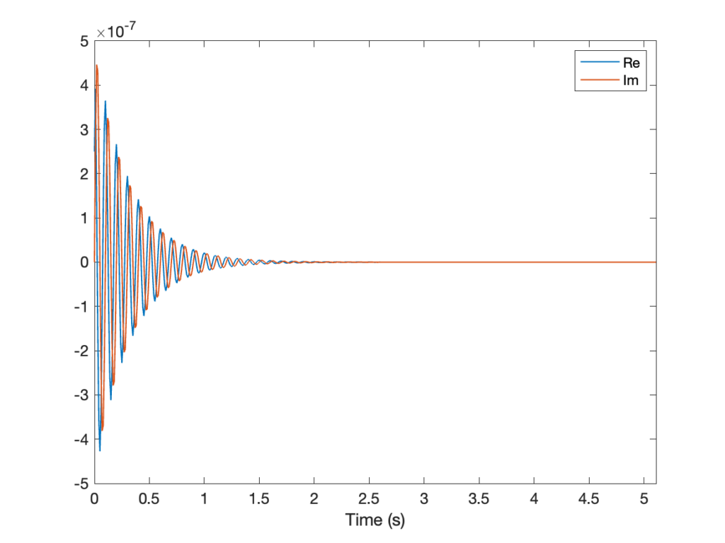

Fourier transform

All we have left to do to get a spectrum is to Fourier transform the FID and generate the corresponding frequency axis. The first and second arguments of the fast Fourier transform function fft are the FID and the desired number of points in the spectrum (i.e., with zero-filling or truncation), respectively. The function fftshift corrects for the fact that fft generates a spectrum where the center of the NMR spectrum appears on the side. fftshift simply reorders the points appropriately.

The frequency of the $k$ ^th point in the spectrum is given by

(17) $\begin{equation*}\nu_k=\frac{k}{L}f,\end{equation*}$

in Hz, with $k\in [-L/2:+L/2-1]$ .

MATLAB
Python

% Fourier transform and phasing:
spc=fftshift(fft(FID,L));

% Frequency axis, Hz
nu = (-L/2:+L/2-1)/L*f;

# Fourier transform and phasing
spc=np.fft.fftshift(np.fft.fft(FID,L));

# Frequency axis, Hz
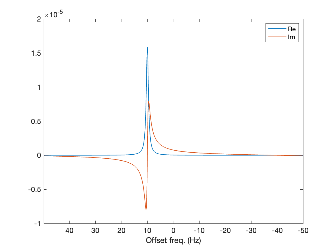
nu = np.arange(-L/2,+L/2)/L*f

Finally, we can plot out first spectrum and see that we go get a signal where we expected it! The plot below shows the real and imaginary components of the spectrum, in blue and red, respectively.

MATLAB
Python

% Visualization of the spectrum
figure(2)
plot(nu,real(spc),'LineWidth',lw), hold on
plot(nu,imag(spc),'LineWidth',lw), hold off
xlabel('Offset freq. (Hz)'), xlim([min(nu) max(nu)])
set(gca,'FontSize',12,'XDir','reverse')

# Visualization of the spectrum
plt.figure(2)
plt.plot(nu,spc.real)
plt.plot(nu,spc.imag)
plt.xlabel('Offset freq. (Hz)')
plt.xlim(np.min(nu),np.max(nu))
plt.legend(['Re','Im'])
plt.gca().invert_xaxis()
plt.show()

Conclusion

We have simulated an NMR using numerical propagation in Liouville space, for the most simple spin system encountered in NMR, i.e., an ensemble of isolated spin 1/2. You can now play with the parameters of the code to see how they affect the results. This is great way to learn without using spectrometer time! If you have a Google account, you can run (and modify) the Python script in your browser without any installation steps. In next posts, we’ll see how adapt this simulation to larger spin system. See you soon!

Simulating a simple 1D NMR spectrum

Experimental vs simulated process

Definition of the variables

Initial state

Excitation pulse

Free evolution propagator

Observable

Free evolution

Apodization

Fourier transform

Conclusion

Leave a Reply Cancel reply

Artist Credit:

Contact:

Website designed and developed by:

Simulating a simple 1D NMR spectrum

Experimental vs simulated process

Definition of the variables

Initial state

Excitation pulse

Free evolution propagator

Observable

Free evolution

Apodization

Fourier transform

Conclusion

Leave a Reply Cancel reply

Artist Credit:

Contact:

Website designed and developed by:

Quantum Insights