March 28th, 2025

Postulate VI – Time evolution (Part II)

Author: Quentin Stern
Editor: Joshua Straub

The full scripts presented in this post are available at these links: MATLAB, Python

In the previous post we saw how the time-dependent Schrödinger equation allows us to calculate how quantum mechanical systems evolve with time, under the effect of the Hamiltonian operator, which describes the total energy of the system. In the case where the Hamiltonian is constant in time, the time-dependent Schrödinger equation can be rewritten in a more convenient form using a time propagation operator or propagator. In this post, we will first show this other form of the Schrödinger equation and where it comes from. Then, we will apply it to the same problem as in the previous post, namely, the evolution of a single spin interacting with a static magnetic field. We will see that the problem is easier and more intuitive using the propagator that the original time-dependent Schrödinger equation.

Time evolution via the propagator

To find the new form the equation of motion, we first calculate the Taylor expansion of the state $\ket{\psi(t)}$ around time $t=0$

(1) $\begin{equation*}\begin{split}\ket{\psi(t)}& =\ket{\psi(0)}+t\frac{d}{dt}\ket{\psi(t)}\Big\vert_{t=0}+\frac{t^2}{2!}\frac{d^2}{dt^2}\ket{\psi(t)}\Big\vert_{t=0}+…\\ &=\sum_{k=0}^{\infty}\frac{t^k}{k!}\frac{d^k}{dt^k}\ket{\psi(t)}\Big\vert_{t=0}.\end{split}\end{equation*}$

Assuming that the Hamiltonian is constant around $t=0$ , we have from the time-dependent Schrödinger equation (using the canonical form in Joules) that

(2) $\begin{equation*}\frac{t^k}{k!}\frac{d^k}{dt^k}\ket{\psi(t)}=\left(-\frac{i}{\hbar}\hat{H}\right)^k\ket{\psi(t)}.\end{equation*}$

Plugging Eq. 2 into Eq. 1, we obtain

(3) $\begin{equation*}\begin{split}\ket{\psi(t)}&=\sum_{k=0}^{\infty}\frac{t^k}{k!}\left(-\frac{i}{\hbar}\hat{H}\right)^k\ket{\psi(0)}\\&=\sum_{k=0}^{\infty}\frac{1}{k!}\left(-\frac{it}{\hbar}\hat{H}\right)^k\ket{\psi(0)}\\&=\exp{\left(-\frac{it}{\hbar}\hat{H}\right)}\ket{\psi(0)},\end{split}\end{equation*}$

where $\exp\left(~\cdot~\right)$ denotes the matrix exponentiation. We now define the time propagation operator or propagator

(4) $\begin{equation*}\begin{split}\hat{U}(t)&=\exp{\left(-\frac{it}{\hbar}\hat{H}\right)}\\&=\sum_{k=0}^{\infty}\frac{1}{k!}\left(-\frac{it}{\hbar}\hat{H}\right)^k,\end{split}\end{equation*}$

and plug it into Eq. 4 to get a convenient form for the Schrödinger equation

(5) $\begin{equation*}\ket{\psi(t)}=\hat{U}(t)\ket{\psi(0)},\end{equation*}$

which describes the evolution of the system using the time derivative of the state only implicitly. If the Hamiltonian is expressed in rad/s, the propagator is

(6) $\begin{equation*}\begin{split}\hat{U}(t)&=\exp{\left(-it\hat{H}\right)}\\&=\sum_{k=0}^{\infty}\frac{1}{k!}\left(-it\hat{H}\right)^k,\end{split}\end{equation*}$

Single spin in a magnetic field

As always, we come back to our favorite example of a single spin interacting with a static magnetic field $B_0$ . The Hamiltonian for this situation is $\hat{H}_0=\omega_0\hat{I}_z$ , expressed in rad/s. The propagator that takes any state of the system from time $0$ to time $t$ is given by

(7) $\begin{equation*}\begin{split}\hat{U}(0\rightarrow t)&=\exp{\left(-it\hat{H_0}\right)}\\&=\exp{\left(-it\omega_0\hat{I}_z\right)}\\ & = \begin{pmatrix} e^{-i\omega_0t/2} & 0 \\ 0 & e^{+i\omega_0t/2} \end{pmatrix}.\end{split}\end{equation*}$

The state of the system as a function of time is then simply obtained by multiplying the state at time $0$ by the propagator of Eq. 7. If the state is initially in state $\ket{\psi(0)}=\ket{x}$ , the state as a function of time is

(8) $\begin{equation*}\begin{split}\ket{\psi(t)} & = \hat{U}(t)\ket{x}\\ & = \begin{pmatrix} e^{-i\omega_0t/2} & 0 \\ 0 & e^{+i\omega_0t/2} \end{pmatrix} \frac{1}{\sqrt{2}}\begin{pmatrix} 1 \\ 1 \end{pmatrix} \\ & = \frac{1}{\sqrt{2}}\begin{pmatrix} e^{-i\omega_0t/2} \\ e^{+i\omega_0t/2} \end{pmatrix}.\end{split}\end{equation*}$

Using the expression for the expectation value of physical observables that we obtained from the fourth postulate, we now calculate the angular momentum along the Cartesians coordinates along time

(9) $\begin{equation*}\begin{split}\braket{\hat{I}_x(t)}&=\braket{\psi(t)\vert \hat{I}_x\vert\psi(t)}\\& = \frac{1}{\sqrt{2}} \begin{pmatrix}e^{+\frac{i\omega_0t}{2}} &e^{-\frac{i\omega_0t}{2}}\end{pmatrix}\frac{1}{2} \begin{pmatrix}0 &1 \\ 1 & 0\end{pmatrix}\frac{1}{\sqrt{2}} \begin{pmatrix}e^{-\frac{i\omega_0t}{2}} \\e^{+\frac{i\omega_0t}{2}}\end{pmatrix}\\&=\frac{1}{4}\begin{pmatrix}e^{+\frac{i\omega_0t}{2}} &e^{-\frac{i\omega_0t}{2}}\end{pmatrix}\begin{pmatrix}e^{+\frac{i\omega_0t}{2}} \\e^{-\frac{i\omega_0t}{2}}\end{pmatrix}\\&=\frac{1}{4}\left(e^{+i\omega_0t}+e^{-i\omega_0t}\right)\\&=\frac{1}{2}\cos\left(\omega_0t\right),\end{split}\end{equation*}$

(10) $\begin{equation*}\begin{split}\braket{\hat{I}_y(t)}&=\braket{\psi(t)\vert \hat{I}_y\vert\psi(t)}\\& = \frac{1}{\sqrt{2}} \begin{pmatrix}e^{+\frac{i\omega_0t}{2}} &e^{-\frac{i\omega_0t}{2}}\end{pmatrix}\frac{1}{2} \begin{pmatrix}0 &-i \\ i & 0\end{pmatrix}\frac{1}{\sqrt{2}} \begin{pmatrix}e^{-\frac{i\omega_0t}{2}} \\e^{+\frac{i\omega_0t}{2}}\end{pmatrix}\\&=\frac{i}{4}\begin{pmatrix}e^{+\frac{i\omega_0t}{2}} &e^{-\frac{i\omega_0t}{2}}\end{pmatrix}\begin{pmatrix}-e^{+\frac{i\omega_0t}{2}} \\+e^{-\frac{i\omega_0t}{2}}\end{pmatrix}\\&=\frac{i}{4}\left(-e^{+i\omega_0t}+e^{-i\omega_0t}\right)\\&=-\frac{i}{2}i\sin\left(\omega_0t\right)\\&=\frac{1}{2}\sin\left(\omega_0t\right),\end{split}\end{equation*}$

and

(11) $\begin{equation*}\begin{split}\braket{\hat{I}_z(t)}&=\braket{\psi(t)\vert \hat{I}_z\vert\psi(t)}\\& = \frac{1}{\sqrt{2}} \begin{pmatrix}e^{+\frac{i\omega_0t}{2}} &e^{-\frac{i\omega_0t}{2}}\end{pmatrix}\frac{1}{2} \begin{pmatrix}1 &0 \\ 0 & -1\end{pmatrix}\frac{1}{\sqrt{2}} \begin{pmatrix}e^{-\frac{i\omega_0t}{2}} \\e^{+\frac{i\omega_0t}{2}}\end{pmatrix}\\&=\frac{1}{4}\begin{pmatrix}e^{+\frac{i\omega_0t}{2}} &e^{-\frac{i\omega_0t}{2}}\end{pmatrix}\begin{pmatrix}+e^{-\frac{i\omega_0t}{2}} \\-e^{+\frac{i\omega_0t}{2}}\end{pmatrix}\\&=\frac{1}{4}\left(1-1\right)\\&=0.\end{split}\end{equation*}$

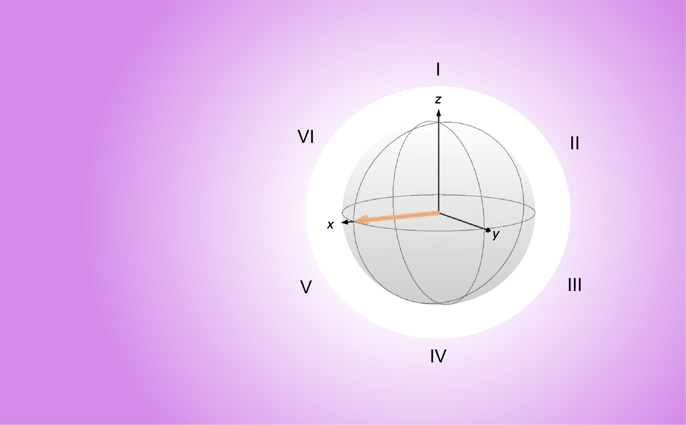
What did we find here? We found a closed solution for the evolution of spin initially perpendicular to a static magnetic field, aligned along the $x$ axis. What this solution tells us is that the spin precesses around the magnetic field in the transverse ( $xy$ ) plane.

Comparison with numerical simulation

This simple case is a nice example to compare analytical results with numerical simulations. We will now implement what we’ve seen in this post as a numerical simulation. We will simulate the evolution of spin initially along the $x$ axis, with a magnetic field along the $z$ axis. We start by choosing some values for the Larmor frequency $\omega_0$ (in rad/s and not in Hz), a time increment $dt$ , and a number of steps $K$ . The reason why we need to define $dt$ and $K$ is that we want to plot the expectation value of the angular momentum as a function of time, which, in the context of numerical simulations, means for a list of discrete values of time.

(12) $\begin{equation*}\begin{split}\hat{U}(dt)^k\ket{\psi_0}&=\hat{U}(kdt)\ket{\psi_0}\\&=\hat{U}(t_k)\ket{\psi_0}\\&=\ket{\psi(t_k)},\end{split}\end{equation*}$

where we used Eq. 6 to go to the last line. This shows that chopping the propagation into smaller time increments yields the same result as performing the propagation in a single step. It’s like saying that waiting 10 times 1 s is the same thing as waiting 1 time 10 s, but using a propagator.

Now, we’ve got all the tools we need to write down the simulation. The code snippet below defines the variables used in the rest of the script. It also defines a time axis $t$ , and an empty matrix in which the results of the numerical simulation will be stored (one row per Cartesian coordinate and one column per time point).

MATLAB
Python
Mathematica

omega0  = 2*pi*1;   % Larmor freq (rad.s-1)
dt      = 0.01;     % Time increments (s)
K       = 300;      % Number of increments (-)

% Time axis and empty vectors to store results 
% of numerical propatation
t       = dt*(0:K-1);
It      = zeros(3,K);

import numpy as np
import matplotlib.pyplot as plt
from scipy.linalg import expm

omega0  = 2 * np.pi * 1  # Larmor freq (rad.s-1)
dt      = 0.01  # Time increments (s)
K       = 300  # Number of increments (-)

# Time axis and empty vectors to store results of numerical propagation
t     = dt * np.arange(K)
It    = np.zeros((3, K))

none

We then compute the initial state $\ket{\psi(0)}$ , the angular momentum operators, the Hamiltonian operator, and the propagator that makes the system move by a time increment $dt$ .

MATLAB
Python
Mathematica

% Initial state
psi0    = [1; 1]/sqrt(2);

% Angular momentum operators
Ix      = [0 1; 1 0]/2;
Iy      = [0 -1i; +1i 0]/2;
Iz      = [+1 0; 0 -1]/2;

% Hamiltonian and propagator during dt
H0      = omega0*Iz;
U0      = expm(-1i*H0*dt);

# Initial state
psi0  = np.array([1, 1]) / np.sqrt(2)

# Angular momentum operators
Ix    = np.array([[0, 1], [1, 0]]) / 2
Iy    = np.array([[0, -1j], [1j, 0]]) / 2
Iz    = np.array([[1, 0], [0, -1]]) / 2

# Hamiltonian and propagator during dt
H0    = omega0 * Iz
U0    = expm(-1j * H0 * dt)

none

The core of the computation happens now. We start by initializing the state of the system by setting the variable describing the system over time $\ket{\psi(t)}$ to the system at time $0$ . Then, at each iteration of the for loop, we compute the expectation value of the angular momentum along the Cartesian coordinates, and store them in the vector we created in the first code block. After that, we “move the system” by a time increment $dt$ .

Note that expectation values are supposed to be real. However, due to the finite precision of numerical calculations, a tiny imaginary component might remain. We discard this small imaginary part by taking the real part of the expectation value before storing it in the matrix.

MATLAB
Python
Mathematica

% Initialization of the system state
psi = psi0;

% Loop for propagation
for k = 1:K
    % Expectation values at time (i-1)*dt
    It(1,k) = real(psi'*Ix*psi);
    It(2,k) = real(psi'*Iy*psi);
    It(3,k) = real(psi'*Iz*psi);

    % Propagation during dt
    psi = U0*psi;
end

# Initialization of the system state
psi   = psi0

# Loop for propagation
for k in range(K):
    # Expectation values at time (k)*dt
    It[0, k] = np.real(np.dot(psi.conj().T, np.dot(Ix, psi)))
    It[1, k] = np.real(np.dot(psi.conj().T, np.dot(Iy, psi)))
    It[2, k] = np.real(np.dot(psi.conj().T, np.dot(Iz, psi)))

    # Propagation during dt
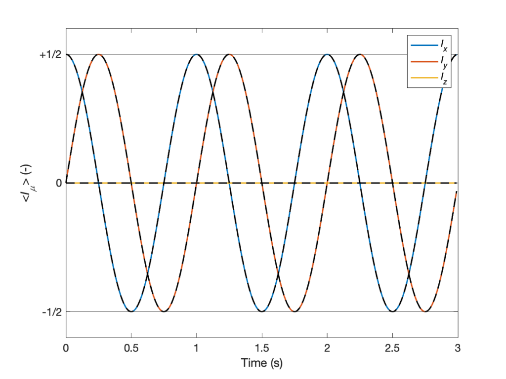
    psi = np.dot(U0, psi)

none

Finally, we compute the analytical solution we obtained in Eqs. 9, 10, and 11, and plot them together with the results of the numerical calculations. The resulting plot is shown below. The results obtained by analytical and numerical calculations are shown as black dashed and solid colored lines, respectively. They match perfectly.

MATLAB
Python
Mathematica

% Analytical solution
Ita = [cos(omega0*t)/2; sin(omega0*t)/2; zeros(1,K)];

% Plot of the results
figure(1), lw = 1.5;
plot(t,It,'LineWidth',lw), hold on
plot(t,Ita,'k--','LineWidth',lw), hold off
yline([+1 -1]/2)
legend({'{\itI_x}','{\itI_y}','{\itI_z}'})
xlabel('Time (s)'), ylabel('<{\itI_\mu}> (-)')
yticks((-1:+1)/2), yticklabels({'-1/2','0','+1/2'})
set(gca,'FontSize',12)

# Analytical solution
Ita   = np.array([np.cos(omega0 * t) / 2, np.sin(omega0 * t) / 2, np.zeros(K)])

# Plot of the results
plt.figure(1)
lw = 1.5
plt.plot(t, It.T, linewidth=lw)
plt.plot(t, Ita.T, 'k--', linewidth=lw)
plt.axhline(y=1/2, color='gray', linestyle='--')
plt.axhline(y=-1/2, color='gray', linestyle='--')
plt.legend(['', '', ''])
plt.xlabel('Time (s)')
plt.ylabel('<> (-)')
plt.yticks(np.arange(-1, 2, 1) / 2, ['-1/2', '0', '+1/2'])
plt.gca().tick_params(labelsize=12)
plt.show()

none

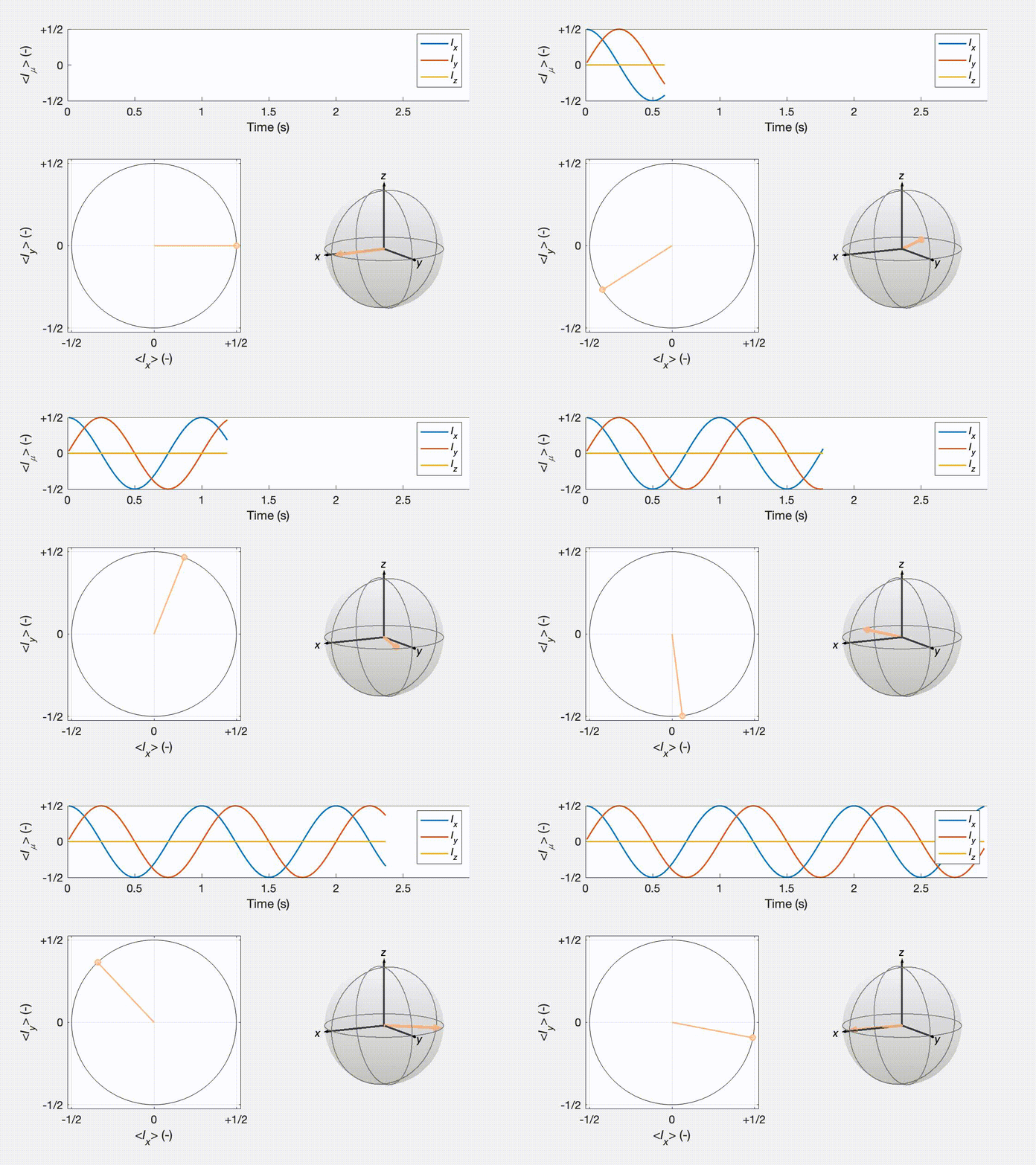
To give a more visual representation of the evolution, we can plot the results dynamically as below. This video was generated using MATLAB. The script is not shown on this page but it is available at the same link as the rest of the scripts.

Conclusion

In this post, we have seen how to redefine the time-dependent Schrödinger equation in terms of a propagator. The equation we derived allows one to compute the state of a quantum mechanical system along time without solving a differential equation, regardless of the initial state of the system. We used this approach to describe the evolution of a spin perpendicular to a static magnetic field both using analytical and numerical computation. The process we have just described is the basis for the simulation of many experiments, even quite sophisticated ones. In fact, in many cases, the process is not much more complicated!

But can it be the end? There must be more to the simulation of magnetic resonance experiments! Yes, there’s a lot more. First, we have only seen how to represent a single spin. We’d need to extend our approach to multiple spins if we want to describe coupled spins. Second, the approach using kets to describe the state of the system only allows us to simulate the dynamics of pure states, while magnetic resonance experiments mostly deal with mixed states or statistical ensemble. To deal with such states, we will need to introduce the density matrix formalism. Still, this will only allow us to describe coherent dynamics, i.e., dynamics of deterministic systems. If we want to include relaxation (which results from stochastic dynamics) in our simulations, we’d need to move to yet another formalism based on superoperators and superkets. Finally, numerical simulation is not everything. There are lots of an other approaches to describe the dynamics of quantum systems. As one out of many examples, Fermi’s golden rule can be used to describe the effect of a small perturbation on a system. It is used a lot, sometimes in complement to numerical simulations.

The list of other approaches to the understanding of magnetic resonance is long but they all have one point in common: they are based on the six postulates we described in this post series. I hope it helped. Stay tuned for more posts on these many topics!

To previous post:
Postulate VI – Part I

Postulate VI – Time evolution (Part II)

Time evolution via the propagator

Single spin in a magnetic field

Comparison with numerical simulation

Conclusion

Leave a Reply Cancel reply

Artist Credit:

Contact:

Website designed and developed by:

Postulate VI – Time evolution (Part II)

Time evolution via the propagator

Single spin in a magnetic field

Comparison with numerical simulation

Conclusion

Leave a Reply Cancel reply

Artist Credit:

Contact:

Website designed and developed by:

Quantum Insights